First Dialogue on RLHF (with a bit of VAE): REINFORCE
P: In which stage can you decompose the most common post-training pipelines?
T: We begin by SFT/IFT (instruction or supervised fine-tuning). The aim is to teach the model to follow QA; in this way, user can ask questions and obtain answer, that is, interact. It turns a next-token predictor (a world model if you wish), into a “persona”. We rely on the same training objective and we focus on a small dataset of high quality examples.

Fig 1., a reward model is a machine that takes text and tells you how good it was.
The second step is RLHF, which aims to improve the style of the answers. We need to teach the model to follow some vague metric of quality, which we cannot compute via a hand-designed function, e.g., how could you define a function over a Kleene Star \(\mathcal V^*\) that returns a scalar proportional to how funny is the message?. Then, we simply use a reward model that is trained to learn our preference and map each model output to its answer
The third step is RLVR, where we boost the actual performance of the model on verifiable domains via more RL training.
P: For example, in which way could RLHF improve the style of the answer of a simple SFT model?
T: Well, for example if I ask to the base model “Who is Franco Battiato?” it would answer directly (“Franco Battiato is the Italian greatest songwriter of 20th century” ) and then start to speak about random topics related to its music until it hits the token max threshold. Instead, the RLHF model would simply give me a synthetic answer.
P: What is the difference between the Superficial Alignment Hypothesis [2] and the Elicitation theory?
T: Both believes that most of the skills are acquired during pertaining. Yet, SAH asserts that you just need few examples to elicit them, and therefore post-training is a tiny and shallow layer on pretraining. Nathan instead believes that skills are grown out from the base model with a lot of effort. He has a more pragmatic view: here is where a lot of money are spent, and even training hours. Here is where we see the core differences between a good and an excellent frontier model. Like in F1, you spend a bit of time at the beginning of the year building the car chassis to be a super cool skeleton, but then you spend a shit ton of time improve aerodynamics and all that boring stuff to beat the other apes competing to go faster than you.
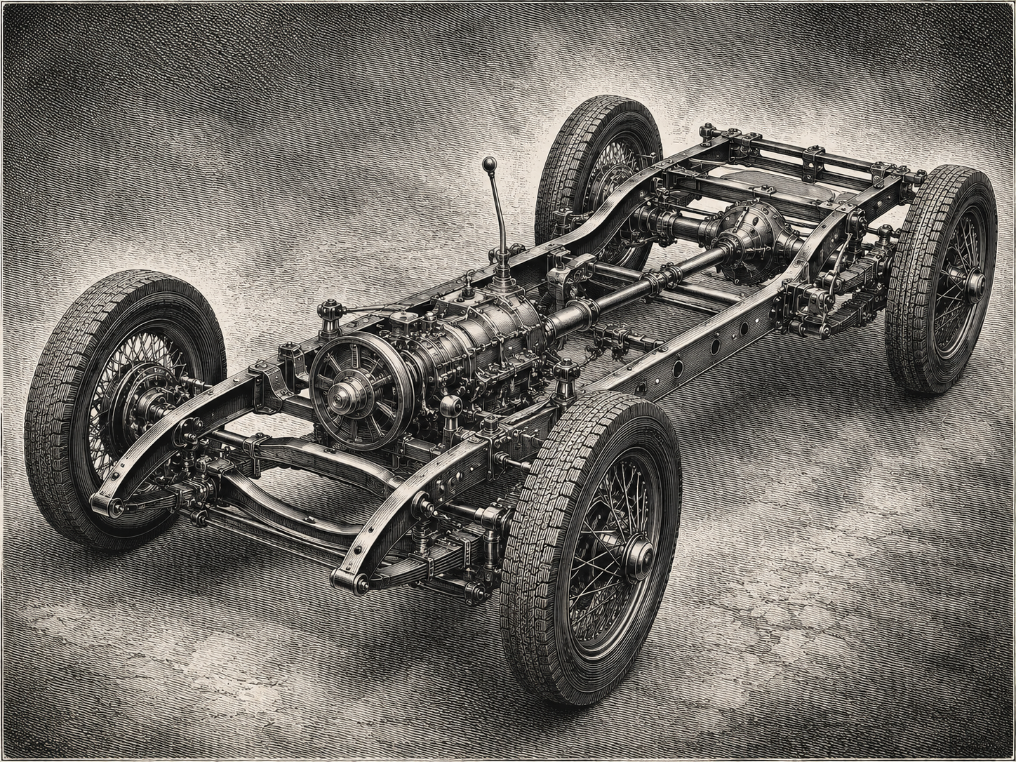
Fig. 2, an image of a car chassis as I had no clue about what it was. I would like to press a button to destroy F1 from the collective memory.
P: why do we need to rely on RL for training during RLHF?
T: Because the reward model has as input a sampled answer from the model:
\[\operatorname{reward} = \operatorname{RM(generated-text)}\]Sampling is not a differentiable function. Yet, there is a known trick in RL to solve this problem: policy gradient methods (REINFORCE).
P: Can you elaborate a bit on the core methodology to differentiate through sampling via
T: Let’s says i have a prompt \(\mathbf c\) and my model, parametrized via \(\theta\), defines a probability distribution on an answer \(\mathbf y \vert \mathbf c\) of other \(t\) token autoregressively:
\[Y | C= \mathbf c \sim\pi_\theta(\mathbf y \mid \mathbf c) = \prod_{t=1}^{T} \pi_\theta(y_t \mid \mathbf c, \mathbf y_{<t})\]Then we have a reward model \(R: \mathcal V^* \to \R\). Ideally, we would like to shakes \(\theta\) via a gradient that maximizes the expected reward (which we approximate via Monte Carlo approximation, that is \(E_{p} [X] \approx \frac 1 n \sum^n_i x_i\) with \(x_i \overset{iid} \sim X\)):
\[J(\theta) = \mathbb{E}_{y \sim \pi_\theta(\cdot \mid \mathbf c)}\big[R(\mathbf y)\big] = \sum_{\mathbf y \in \mathcal{V}^T} \pi_\theta(\mathbf y \mid \mathbf c)\, R(\mathbf y)\]Here you can see the problem clearly:
...
logits = policy(prompt)          # all good we can backprop.
y = sample(logits)               # fook we cannot backprop. (+ discrete!)
reward = RM(y)                   # all good... but gradient arrives dead.
...
Connection with VAE
This is similar to the problem we have with VAE. There we need the reparametrization trick as we cannot back-propagate via a gaussian:
...
mu, sigma = encoder(x) # all good we can backprop.
z = random.normal(mu,sigma) # fook we cannot backprop.
x_recon = decoder(z) # all good we can backgrop.
This was solved via the reparametrization which isolate the sampling in a branch where our gradient does not flow backwards via backpropagation
...
mu, sigma = encoder(x) # all good we can backprop.
e = random.normal(0,I) # we do not care
z = mu + e*sigma # all good now
x_recon = decoder(z) # all good we can backgrop.
Then what is the solution? We do not have a clean trick as the reparametrization trick, where we can keep the same flow and just change its computation instantiation. With REINFORCE (policy gradient), we change what we differentiate for, yet it works! Check this out:
...
y = sample(logits)               # we do not care (no grad through this branch)
reward = RM(y).detach()          # we do not care (just a constant)
logp = log_prob(policy(prompt), y)   # all good we can backprop.
loss = -reward * logp            # all good — Adam on this.
...
The core idea is that we stop optimizing \(\theta\) to improve the expected reward of its answer directly. Instead, we try to optimize \(\theta\) to increase the probability of answer that have good reward. In practice, we say:
- stop doing this: “sample y, compute R(y), call
.backward()on R.” - start doing this: “sample y, compute R(y), call
.backward()on-R·log πθ(y).”
On the one hand, this is now possible as the gradient is inside the sampling, so we can simply kill the sampling part via a monte carlo approximation. On the other hand, this core identity \(\nabla_\theta \pi_\theta = \pi_\theta \, \nabla_\theta \log \pi_\theta\) shows us that is the same (do not be scare it is the classic \(\frac{d \log f(x)} {dx} = \frac 1 x \frac{d f(x)} {d x}\to \frac{d f(x)} {d x} = x\frac{d \log f(x)} {dx}\)):
\[\underbrace{\nabla_\theta\, \mathbb{E}_{\mathbf y \sim \pi_\theta}\big[R(\mathbf y)\big]}_{\text{the gradient of the true objective}} = \mathbb{E}_{\mathbf y \sim \pi_\theta}\Big[\underbrace{R(\mathbf y)\,\nabla_\theta \log \pi_\theta(\mathbf y)}_{\text{what recipe B computes per sample}}\Big] \approx \frac 1 N \sum_{\mathbf y \sim \pi_\theta}\Big[\underbrace{R(\mathbf y)\,\nabla_\theta \log \pi_\theta(\mathbf y)}_{\text{what recipe B computes per sample}}\Big]\]A closing remark: the reason why this new objective is equivalent to optimize the weights with steps that increase chance of good samples, is that is is a weighted sum where the weights are given via \(R(\mathbf y)\). If I am trying to optimize \(\mathcal L = \mathbf c^{\top} f_{\theta}(\mathbf y)\) by linearity of differentiation my gradient will be:
\[\nabla_\theta \mathcal{L} = \mathbf{c}^\top \nabla_\theta f_\theta(\mathbf{y}) = \sum_{i} c_i \, \nabla_\theta \big[f_\theta(\mathbf{y})\big]_i\]Therefore I will move a lot in the directions \(\big[f_\theta(\mathbf{y})\big]_i\) where \(c_i \approx 1\) (is very high), and a little when \(c_i \approx 0\) (is very little)