Notes on Diffusion Models
A. Denoising Diffusion Probabilistic Models (DDPMs)
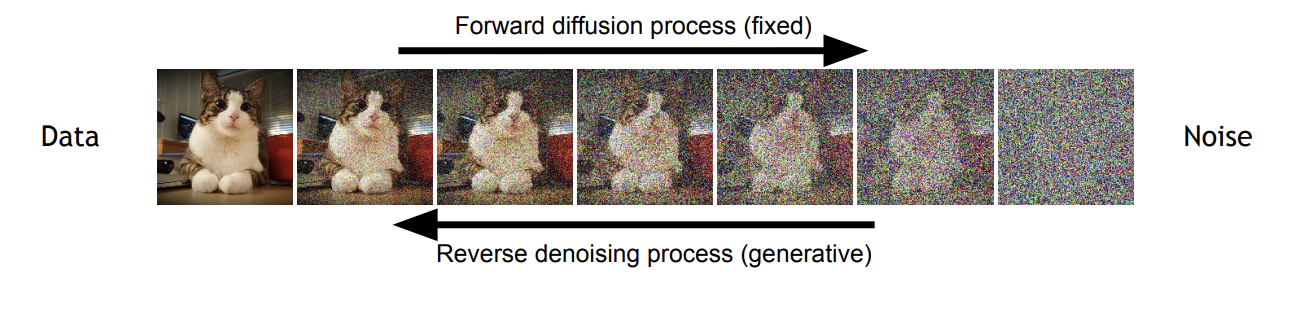
Diffusion models consist of two process. A fixed forward process where you add gaussian noise to input image, a learned reverse process where you remove noise.
1. The Forward Process: Mathematical Definition
The forward process is a fixed Markov chain that adds Gaussian noise according to a pre-defined variance schedule \(β_t\)
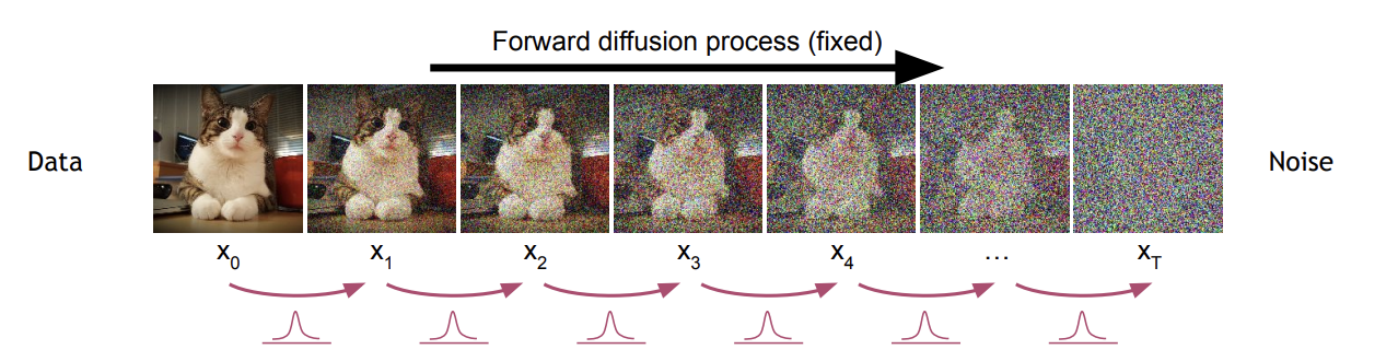
SINGLE STEP TRANSITION The transition from one timestep to the next is defined as a Gaussian distribution where the mean is a scaled version of the previous state \(x_{t-1}\) and the variance is fixed by the schedule \(\beta_t\) s.t. \(t \to T\) then \(\beta_t : 0 \to 1\)
\[q(x_t|x_{t-1}) = \mathcal{N}(x_t; \sqrt{1-\beta_t} x_{t-1}, \beta_t \mathbf{I})\]JOINT DISTRIBUTION Given that we have a markovian structure we can simply define the joint distribution:
\[q(x_0,...,x_t) = q(x_0)\prod_tq(x_t | x_{t-1})\]CLOSED FORM t-STEP MARGINAL A key result is that \(x_t \vert x_0\) has a closed gaussian form. This means we can sample \(x_1,...,x_T\) in parallel and is super-useful to speed up training

In practice we sample from it via the reparametrization trick that makes us write:
\[x_t = \sqrt{\bar{\alpha}_t }x_0+ \sqrt{(1-\bar{\alpha}_t )}\epsilon \;\;\;\; \epsilon \sim N(0,I)\]Which means we just need to compute alpha, take the original image and sample \(\epsilon\).
NB here the coefficient \(\bar{\alpha}_t\) is opposite to \(\beta_t\). While \(\beta_t\) is increasing and \(\beta_0 = 0\) instead \(\bar{\alpha}_t\) is decreasing and \(\bar{\alpha}_T=0\)
DERIVING CLOSED FORM GAUSSIAN To derive the close form gaussian set \(\alpha_t = (1-\beta_t)\) as a useful short hand and start by using the reparametrization trick to write \(q(x_t \vert x_{t-1})\):
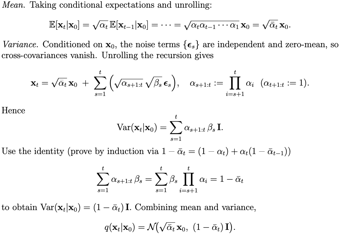
\[x_t = \sqrt{{\alpha} }x_{t-1}+ \sqrt{\beta_t }\epsilon \;\;\;\; \epsilon \sim N(0,I)\]Now by linearity of gaussian we know that the all the \(x_t \vert x_0\) will be gaussian, so we just unroll the mean and the variance to learn them
solution
IMPORTANCE OF GAUSSIANITY The choice of Gaussian noise is not arbitrary; gaussian maps been closed under sum, linear maps…allow for the simple, closed-form expressions for:
- the forward marginal \(q(x_t \vert x_0)\)
- the forward posterior \(q(x_{t-1} \vert x_t, x_0)\) →
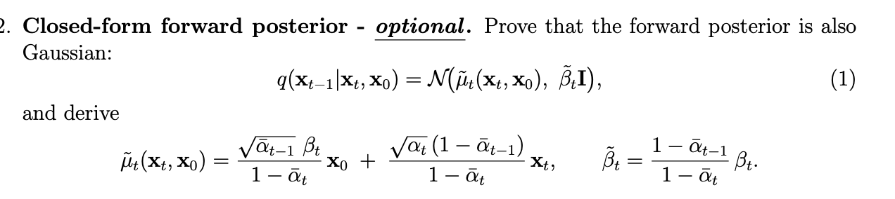
If another noise distribution like Laplace or uniform were used, these elegant closed forms would not exist, making the training objective (the ELBO terms) and the sampling updates intractable.
2. The Reverse Process and Training Objective
Now that we saw how to generate noisier image in the forward pass we want to learn the true reverse pass to generate denoised image. That is we want to learn \(\theta\) such that our parametrized distribution \(p_{\theta}\) is similar to the true reverse process \(p\):
\[p_θ(x_{0:T})=p(x_T)∏^T_tp_θ(x_{t−1}∣x_t) \approx p(x_T)∏^T_tp(x_{t−1}∣x_t) = p(x_{0:T})\]WHY LEARN ? INTRACTABILITY OF REVERSE The main problem of denoising is that \(x_{t-1} \sim q(x_{t-1} \vert x_t)\) is intractable. So we cannot compute it simply as in the forward process and we need to learn

LEARNING PROBLEM The goal of training in the reverse process is to learn a neural network \(p_θ\) that can approximate the true reverse denoising distribution. So we could try to maximize the likelihood of real data \(x_0\) under our parametrization \(p_{\theta}\) but we cannot compute such distribution! but we can do ELBO!
ELBO Training aims to maximize the log-likelihood of the data, log pθ(x₀), which is computationally intractable. Instead, we maximize a tractable lower bound, the Evidence Lower Bound (ELBO). For diffusion models, the negative log-likelihood can be bounded by a sum of Kullback-Leibler (KL) divergence terms:
This can be written more compactly as \(≤ L_T + Σ_{t=2}^T L_{t-1} + L_0\). Minimizing this loss is equivalent to making the learned reverse distribution pθ match the true (but intractable) reverse distribution q. Each of these terms has a meaning:

THE LOSS TERMS \(L_{t-1}\) The core of the training involves minimizing the \(L_{t-1}\) term. I_f we assume the learned reverse process_ \(p_θ\) is also Gaussian with a learned mean \(µ_θ(x_t, x_0)\) and a fixed variance \(σ²_t*I\)
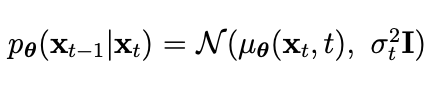
then the KL divergence simplifies significantly. It becomes an MSE term between the predicted reverse mean µ_θ and the true forward posterior mean \(µ̃_t\), plus constants that do not depend on µ_θ:
\[L_{t-1} = \mathbb{E} \left[ \frac{1}{2\sigma_t^2} || \mu_\theta(x_t, t) - \tilde{\mu}_t(x_t, x_0) ||_2^2 \right] + \text{const}\]SIMPLIFYING \(L_{t-1}\) FURTHER VIA \(\epsilon\) Start from the the reparametrization of the t-step forward marginal:
\[x_t = \sqrt{\bar{\alpha}_t }x_0+ \sqrt{(1-\bar{\alpha}_t )}\epsilon \;\;\;\; \epsilon \sim N(0,I)\]Then notice this implies:
\[x_0 = \frac{(x_t - \sqrt{1-\bar{\alpha_t}}\epsilon)}{\sqrt{\bar{\alpha_t}}}\]Now remember that the forward posterior mean is:

So by using both we arrive to:
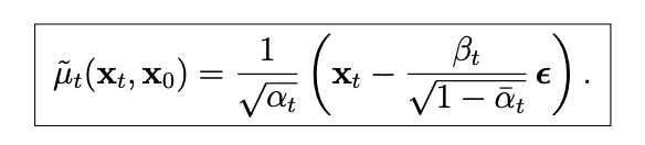
If now we choose our parametrization for \(\mu_{\theta}\) (we can do whatever we want with it) as:

Then \(L_{t-1}\) simplifies to

Proof
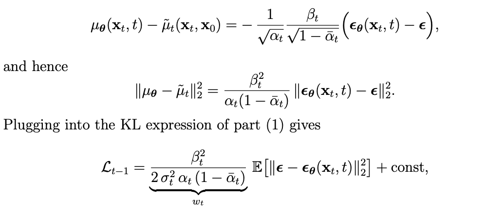
DROP WEIGHT \(w_t\) While the ELBO provides a theoretically sound objective, a simplified version having only the expectation term \(L_{t-1}^{simple} =\mathbb{E}[ \vert \epsilon - \epsilon_\theta(x_t, t) \vert _2^2 ]\) often yields better practical results.
- Rebalancing toward hard regimes: It gives uniform emphasis to all timesteps, forcing the model to become accurate in the highest-noise regimes where reverse sampling begins, which is crucial for forming the sample’s global structure.
- Lowering loss-scale variation: It removes per-step loss scaling differences from the
βtschedule, which can stabilize optimization. - Improving empirical quality: Although it no longer optimizes a tight likelihood bound, the uniform emphasis empirically improves perceptual metrics like FID.
3. Sampling Process Via Ancestral Sampling
Once the noise prediction network ϵ_θ is trained, we can generate new samples using an iterative ancestral sampling process.
UPDATE RULES Starting from pure noise \(x_T ~ N(0, I)\), we iterate backward from \(t=T\) to \(t=1\). Each step \(x_{t-1}\) is sampled from the learned reverse distribution \(p_θ(x_{t-1} \vert x_t).\) Using the ϵ-prediction parameterization, the update step is:

TWO CHOICE FROM AMOUNT OF STOCHASTICITY \(σ_t\). The term \(σ_t\) controls the amount of stochasticity in the reverse step. There are two common choices:
- \(σ_t = √β_t\): This choice injects more noise, leading to higher variance and diversity.
- \(σt = √β̃_t\): This choice, derived from the true posterior variance, injects less noise. It produces sharper, lower-variance samples but relies more heavily on the network’s accuracy.
This represents a bias-variance trade-off between diversity (higher σt) and fidelity (lower σt).
FINAL IMAGE ESTIMATOR At any timestep \(t\), we can get an estimate of the final clean image \(x_₀\) by rearranging the forward process t- step reparameterization and replacing the unknown true noise ϵ with the network’s prediction ϵ_θ. Start from here:
\[x_t = \sqrt{\bar{\alpha}_t }x_0+ \sqrt{(1-\bar{\alpha}_t )}\epsilon \;\;\;\; \epsilon \sim N(0,I)\]extract \(x_0\):
\[x_0 = \frac{(x_t - \sqrt{1-\bar{\alpha_t}}\epsilon)}{\sqrt{\bar{\alpha_t}}}\]substitute \(\epsilon \to \epsilon_{\theta}\):

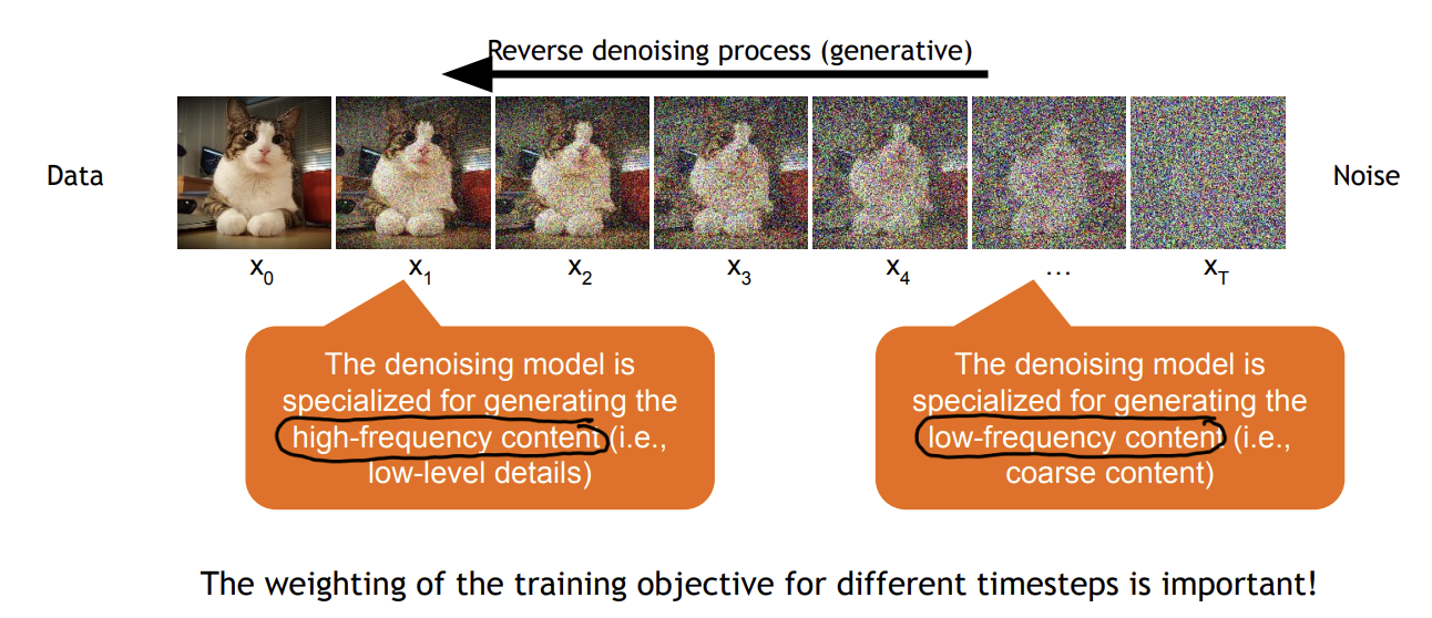
4. Additional: Content-Detail Tradeoff
B. The SDE Framework: A Continuous-Time Perspective
1. Introduction: Generalizing to Continuous Time
The discrete-time DDPM process can be viewed as a numerical discretization of a continuous-time Stochastic Differential Equation (SDE). Adopting this perspective provides a more general mathematical foundation that unifies different diffusion model variants and opens the door to more flexible and powerful sampling methods.
2. SDE BACKGROUND
An ordinary differential equations can be euler approximated via:
\[x(t+\Delta t) \approx x(t)+f(x(t),t) \Delta t\]Here it tells you that your particle at time \(t+\Delta t\) will be in the previous position + a drift term defined by \(f(position,time)\). An SDE is the same but it adds a random increment on top:
\[x(t+\Delta t) \approx x(t)+f(x(t),t) \Delta t + g(t) \sqrt{\Delta t} \epsilon \;\;\; \epsilon \sim N(0,I)\]So the next position does not depend only on the drift but also on a random steps (diffusion term). If we want to know the actual SDE rather than this approximation we just need to pull the \(\Delta_t \to dt\) by making the step very small and we get a Wiener (Brownian) Process:
\[dx_t = f(x_t,t)dt + g(t)dW_t\]The Wiener process is a sequence of rv has the charactersitic distribution:
\[\{W_i\}_{i\ge 0}\ \text{s.t.}\ W_j - W_k \sim \mathcal{N}(0,\ j-k)\]So that:
\[dW_t \approx W_{t+dt}-W_t \sim \mathcal{N}(0,\ dt)\]3. Forward Diffusion
By considering an infinitesimally small time step and applying a first-order Taylor expansion to the discrete forward step, we can derive the continuous-time forward SDE.
\[dx_t = -\frac{1}{2} \beta(t) x_t dt + \sqrt{\beta(t)} dW_t\]- DRIFT TERM \(-\frac{1}{2} \beta(t) x_t\) is the drift term, which pulls the state toward the origin
- DIFFUSION TERM \(\sqrt{\beta(t)}\) is the diffusion term, which controls the magnitude of the random noise \(dW_t\) (a Wiener process).
GAUSSIANITY OF t-STEP FORWAD A very cool step of using this diffusion sde for the noising forward process is that we get a gaussian t-step forward process:
\[q(x_t|x_0) = N(\alpha_tx_0, \sigma^2I)\]With \(\alpha_t = \exp\!\left(-\frac{1}{2}\int_{0}^{t}\beta(s)\,ds\right), \qquad\sigma_t^{2} = 1 - \alpha_t^{2}.\) This allow us to sample directly in one shot the diffusion output:
\[x_t = \alpha_t x_0 + \sigma_t \epsilon, \qquad \epsilon \sim \mathcal{N}(0, I).\]4. Reverse Diffusion
A key result in stochastic calculus shows that any diffusion process has a corresponding reverse-time SDE. The general form is:
\[d_{x_t} = [ f(x_t, t) - g(t)²∇_{x_t} log(q_t(x_t)) ] dt + g(t) dW_t\]For our specific SDE, this becomes
\[dx_t = \left[ -\frac{1}{2} \beta(t)x_t - \beta(t)\nabla_{x_t} \log q_t(x_t) \right] dt + \sqrt{\beta(t)} dW_t\]his equation has two main components in its drift term:
- FORWARD DRIFT TERM the original forward drift \(f(x_t, t) = -\frac{1}{2} \beta(t)x_t\)
- CORRECTION TERM crucial correction term involving the score function \(\beta(t)\nabla_{x_t} \log q_t(x_t)\)where \(g(t)= \beta(t)\) ,
∇xt log qt(xt), which steers the sampling process toward high-density regions of the true data distribution.
5. Denoising Score Matching
To use the reverse SDE for generation (reverse process), we must know the score function \(\nabla_{x_t} \log q_t(x_t)\). Indeed, is the only uknown in the reverse process formula, as we do define in the forward the drift term \(\beta(t)\) ourselves. We can learn it via a neural network \(s_{\theta}\).
INTRACTABILITY OF MARGINAL SCORE. Directly learning the marginal score is intractable:
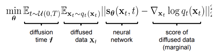
The key reason why is intractable is that we cannot compute \(q_t(x_t)\) as, to do so, we need to compute \(q_t(x_t) = ∫ q_t(x_t \vert x_0)q_0(x_0)dx_0\) which is a is a complex mixture over the entire dataset, making its score computationally infeasible. Indeed, one can show that the score is equal to this via the Fisher Identites:

Now while the conditional score \(\nabla_{x_t} \log q_t(x_t \vert x_0)\) is closed form as \(q_t(x_t \vert x_0)\) is gaussian (showed above), the expectation is on a distribution we do not know and is intractable \(q(x_0 \vert x_t)\) (if we knew it we could directly generate with it )
Proof
Open the derivative + law of total probability

Leibniz rule interchange integral and delta
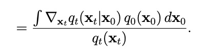
Use the log trick to rewrite the delta of prob distribution

CONDITIONAL SCORE LEARNING The key insight of Denoising Score Matching (DSM) is to sidestep this problem. Instead of training a model on the intractable marginal score, we train it on the tractable conditional score: \(\nabla_{x_t} \log q_t(x_t \vert x_0)\). Indeed, if you learn the score \(\hat{y}\) over (x,y) your optimal y is \(y^* = E[Y \vert X=x]\). Therefore, if you learn the score \(s_{\theta} \to s^*\) is like you learn an expectation of that output for a given input:
\[s^*(x_t,t)= \mathbb{E}\!\left[\nabla_{x_t}\log q_t(x_t\mid x_0)\ \big|\ x_t\right]\]But by the fisher identity:
\[\nabla_{x_t}\log q_t(x_t)= \mathbb{E}\!\left[\nabla_{x_t}\log q_t(x_t\mid x_0)\ \big|\ x_t\right].\]Therefore:
\[s^*(x_t,t)=\nabla_{x_t}\log q_t(x_t).\]LEARNABILITY OF CONDITIONAL SCORE Now the conditional score is much easier to learn as we target this

This is easier because thanks to the gaussianity of \(q_t(x_t \vert x_0)\) we can rewrite the conditional score in a closed form:
\[\nabla_{x_t}\log q_t(x_t\mid x_0)= -\frac{1}{\sigma_t^{2}}\left(x_t-\alpha_t x_0\right).\]Now we saw that the forward t-step marginal can be written as:
\[x_t = \alpha_t x_0 + \sigma_t \epsilon, \qquad \epsilon \sim \mathcal{N}(0, I).\]Therefore, we can plug this formula into \(\frac{1}{\sigma_t^{2}}\left(x_t-\alpha_t x_0\right)\) and we get that the conditional score is:

Now if we make an extra step and we parametrize the score predictor to be a function of the noise:
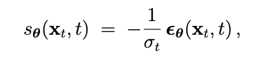
We get the same predictor of the \(L_{t-1}\) of the previous chapter:

SAMPLING Once we trained \(s_{\theta}\) or \(\epsilon_{\theta}\) we can simply plug them in the reverse drift and generate:
\[dx_t = \left[ -\frac{1}{2} \beta(t)x_t - \beta(t)s_{\theta}(x_T) \right] dt + \sqrt{\beta(t)} dW_t\]C. Modern Architectures and Techniques
4.1. Introduction: From Theory to Practice
This section covers the key architectural components and advanced techniques that have enabled diffusion models to achieve state-of-the-art performance, moving from the foundational theory to practical, high-performance implementations.
4.2. Core Architectural Components
- Backbone: The neural network architecture for the denoising model is typically a U-Net or a Denoising Autoencoder. The U-Net’s skip connections are particularly effective at preserving high-resolution details.
- Time Representation: The diffusion timestep
tis a critical input, telling the model how much noise to expect. It is typically encoded into a high-dimensional representation using sinusoidal positional embeddings or random Fourier features, which are then integrated into the network’s residual blocks. - Diffusion Transformers (DiT): More recent architectures have replaced the convolutional U-Net with a Vision Transformer (ViT). The noisy image is broken down into a sequence of tokenized patches, and the Transformer operates on this sequence to predict the denoised patches, much like an LLM operates on text.
4.3. Achieving Controllable Generation
To guide generation toward specific concepts (e.g., a text prompt), guidance techniques are essential. The basis for these techniques is the unconditional score sθ(xt).
Step 1: Classifier Guidance. This technique uses a separate, pre-trained classifier pφ(y|xt) to steer the diffusion process. At each sampling step, the score is modified by adding the gradient of the classifier’s log-probability, effectively pushing the sample xt to be more recognizable as the desired class y. The guided score is approximated as: s_\theta(x_t) + \nabla_{x_t} \log p_\phi(y|x_t)
Step 2: Classifier-Free Guidance (CFG). A more modern and widely used technique, CFG eliminates the need for an external classifier. It relies on a single conditional diffusion model trained on both conditional and unconditional inputs (by randomly dropping the conditioning information during training). During sampling, the final score is an extrapolation away from the unconditional score and towards the conditional score, creating an “implicit classifier” from the diffusion model itself.
4.4. Improving Efficiency with Latent Diffusion
Running the diffusion process on high-resolution images is computationally expensive. Latent Diffusion Models (LDMs), such as Stable Diffusion, solve this by performing diffusion in a much smaller, compressed latent space. This is a two-stage process:
- Train an Autoencoder: A powerful convolutional autoencoder is trained first. The encoder maps a high-resolution image to a low-dimensional latent representation, and the decoder reconstructs the image from this latent.
- Run Diffusion in Latent Space: The entire forward (noising) and reverse (denoising) diffusion process is then performed on these compact latent embeddings. This approach is significantly more computationally efficient, enabling faster training and inference.
4.5. Flow Matching: An Alternative View
Flow Matching has emerged as a conceptually simpler alternative to diffusion models. Instead of defining a forward noising SDE, it directly learns the vector field required to interpolate between a simple noise distribution and the target data distribution. It has been shown to be equivalent to diffusion for certain configurations but is often praised for its implementation simplicity, as it avoids the need for SDEs and score matching.
D. Comparisons
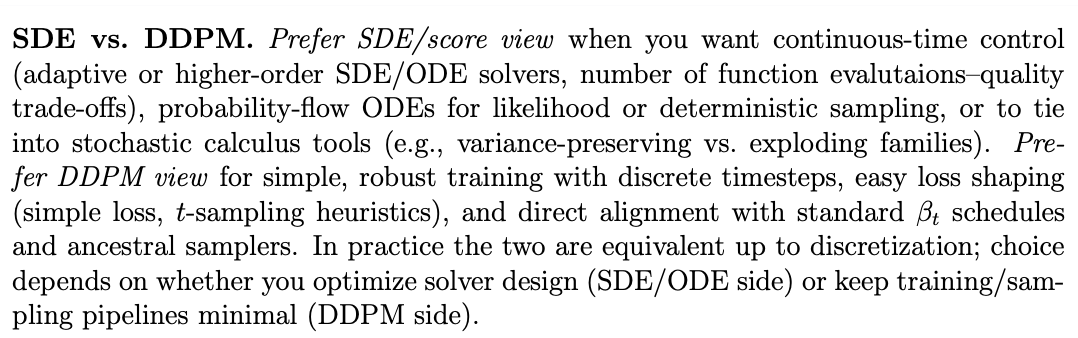
5.2. DDPM vs. SDE/Score Perspective
| Feature | DDPM View (Discrete) | SDE/Score View (Continuous) |
|---|---|---|
| Time Domain | Operates on a fixed, discrete set of timesteps t = 1, ..., T. | Operates in continuous time t ∈ [0, T]. |
| Training Simplicity | Training is very straightforward with discrete schedules and simple loss weighting schemes. | Provides a deeper theoretical connection to stochastic calculus and score-based modeling. |
| Sampling Flexibility | Primarily uses the ancestral sampler, with limited flexibility in step size. | Enables the use of a wide variety of advanced SDE and ODE solvers, allowing for trade-offs between speed and quality. |
5.3. Diffusion Models vs. VAEs
While diffusion models can be seen as a type of hierarchical VAE, they have several key distinguishing features:
- Encoder: The “encoder” in a diffusion model (the forward noising process) is fixed and non-learnable, whereas a VAE learns its encoder.
- Latent Space: The latent variables (
x₁, ..., xT) in a diffusion model have the same dimension as the input datax₀. - Network: A single denoising neural network’s parameters are shared across all timesteps
t. - Prior: The forward process converges to a simple Normal distribution by construction, effectively avoiding the “prior holes” or “posterior collapse” issues that can affect VAEs.
5.4. The Frequency Domain Perspective
The noising and denoising processes can be understood from a frequency perspective:
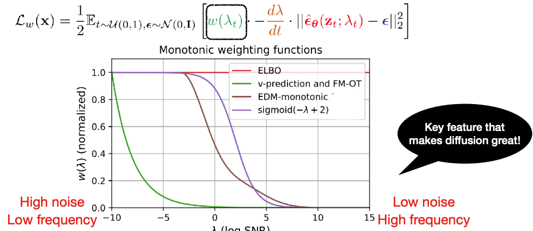
- Forward Process: When adding noise, high-frequency content (fine details, textures) is destroyed much more quickly than low-frequency content (overall shapes, coarse structure).
-
Reverse Process: Consequently, the denoising network learns to generate content in a coarse-to-fine manner. At high-noise timesteps (large
t), the model focuses on generating the robust, low-frequency structure of the image. As sampling proceeds to low-noise timesteps (smallt), the model refines this structure by adding high-frequency details._ _ \|...\| \| \| ____\| \|____ \| \| \| \| \|____\| \|____\| nergo
Diffusions applications
Reweighted ELBO allows diffusion models to spend more capacity on low-frequency components (meaning more semantical aspects instead of the minute details)
Latent diffusion models
The idea of having latent diffusion models allows the diffusion process to denoise in latent hence focussing on large-scale image structure (the semantics of the image), while having an autoencoder + GAN only generating local details.
REPA
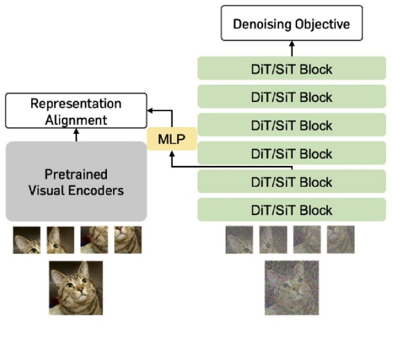
Modern approaches like Diffusion Transformers scale effectively with compute and model size.
Representation Alignment (REPA) align the diffusion model’s intermediate features with pretrained perceptual visual encoders. This alignment allows the model to leverage perceptual inductive biases, resulting in training that is up to 17.5 times faster
Generative Learning Trilemma
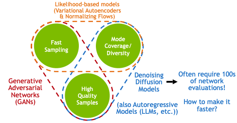
GANs are fast and high quality but suffer mode collapse.
VAE are fast and have good mode coverage but low quality.
Diffusino models are high quality and have good mode coverage but are very slow.
three main approaches to accelerate diffusion:
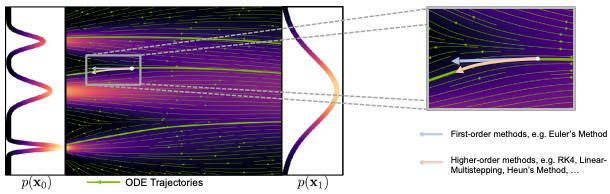
- Fast ODE/SDE Solvers: Because the sampling process involves iterative steps, advanced solvers (like DPM-Solver++ or Heun’s Method) can approximate the Ordinary Differential Equation (ODE) trajectories more efficiently, reducing the number of steps required (e.g., from hundreds down to 15-20 steps).
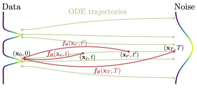
- Trajectory Distillation: This method learns a function that reproduces the multi-step mapping of a teacher model in a single step (e.g., consistency models). While it provides a one-to-one mapping, it is difficult to reduce the process to very few steps.
-
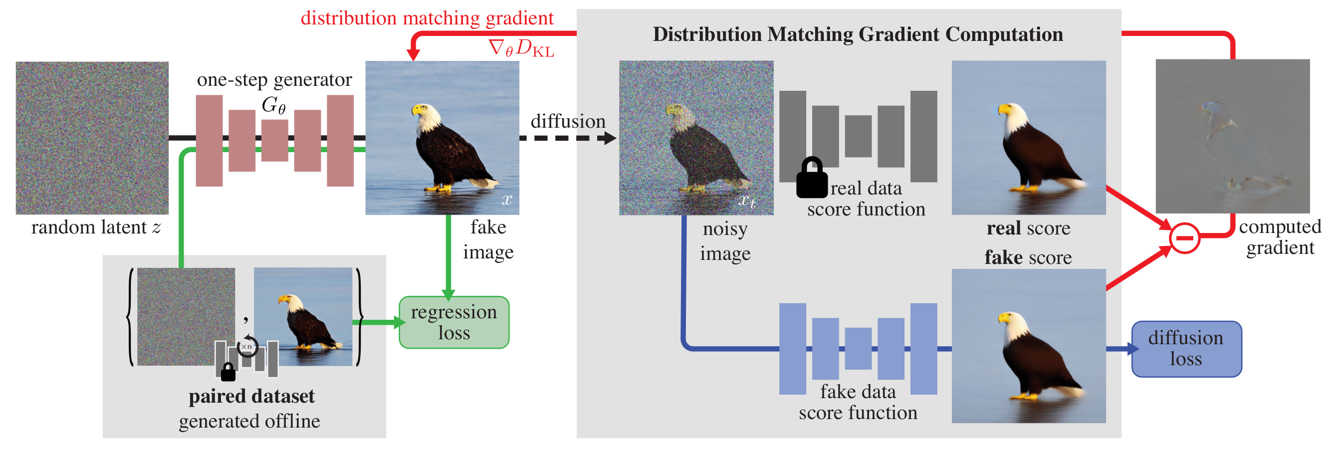
Variational Distillation: This approach matches the student model’s distribution to the teacher’s via a variational objective (VDKL). It enables very fast, one-step generation but incurs extra compute costs and risks mode collapse. The core idea of DMD distillation is to minimize the KL divergence between the output distributions of the distilled model and the original model