Notes on Transformers

0. Prerequisite: A Mental Model for Vector and Matrix Algebra

0.1 Vector Dot Product \(u^Tv\)

REQUIREMENTS The dot product between two vector requires that \(u,v\) have the same dimension \(d\).

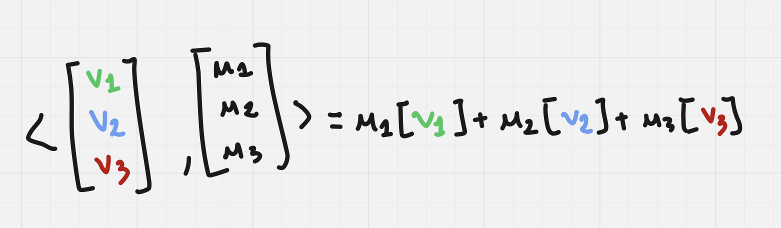
\(u^Tv\) the vector dot product \(u^Tv = <u,v>\) is a linear combination of the entry of \(v\) via the entry of \(u\) as weights. It is just an unscaled similarity mechanism between two vector from the same vector space

0.2 Matrix Left Vector Multiplication \(Av\)

REQUIREMENTS The number of columns of \(A\) must match the number of entries of \(v\), that is \(A \in R^{ r \times d}, v \in R^r\).

\(Av\) is just a linear combination of the column of A with the entries of v. So, when \(v \in \Delta\) it is an column averaging mechanism.

0.3 Matrix Right Vector Multiplication \(u^TA\)

REQUIREMENTS The number of rows of \(A\) must match the number of entries of \(u\), that is \(A \in R^{ d \times c}, u \in R^d\)

\(u^TA\) is just a linear combination of the rows of A. So, when \(u \in \Delta\) it is an row averaging mechanism.

0.4 Matrix Matrix Multiplication \(AB\)

The main mental model is the rlcr-model (Red Lions Chase Rabbits), that is row from left columns from right. This is because both for the requirements and the calculation we will all time care about rows from A and columns from B

REQUIREMENTS The dimension of the rows of A (rl) must match the dimension of the columns of B (cr). As “dimension of row of A = number of columns of A” and “dimensions of columns of B = numbers of rows of B” we have \(A \in R^{ r,d}, B \in R^{d,c} \to C^{r,c}\)

To compute think to \(C=AB\) we should start from \(C\):

• ENTRY-WISE \(C_{i,j} = A_{i,.}B_{.,j}\) is a dot product between the \(i^{th}\) row of A and the \(j^{th}\) column of B. So, C is a database of similarities between A rows and C columns
• for the row/columns wise view start from the rlcr to identify if we use a row of A or a column of B and after use the full same set of entities from the other matrix
  • ROW-WISE \(C_{i,.} = A_{i,.}B\) is the \(i^{th}\) row of A used in a Matrix Right Vector multiplication of rows of B. That is, we use the row of A to average the rows of B
  • COLUMN-WISE \(C_{.,j} = A B_{.,j}\) is the \(j^{th}\) column of B used in a Matrix Left Vector multiplication of columns of A. That is, we use the column of B to average the columns of A

SPECIAL CASE \(A^TA\) In this case C is a symmetric database of similarities between columns of A

• Indeed, \(C_{i,j}\) is the \(j^{th}\) column of A dot product with the \(i^{th}\) row of \(A^T\) so the \(i^{th}\) column of A
• \(C_{.,j} = C_{j,.}\) and it is obtained by Matrix Left Vector Multiplication of \(j^{th}\) column of A with

1. Autoregressive Transformers From Scratch (N5)

Assume you want a function to generate MNIST-like images of digits. A simple option is to train an autoregressive transformer. The core idea is that we can think as a sequence of patches.

1.1 Patches

The process of turning images into patches means getting a big image into a sequence of small images

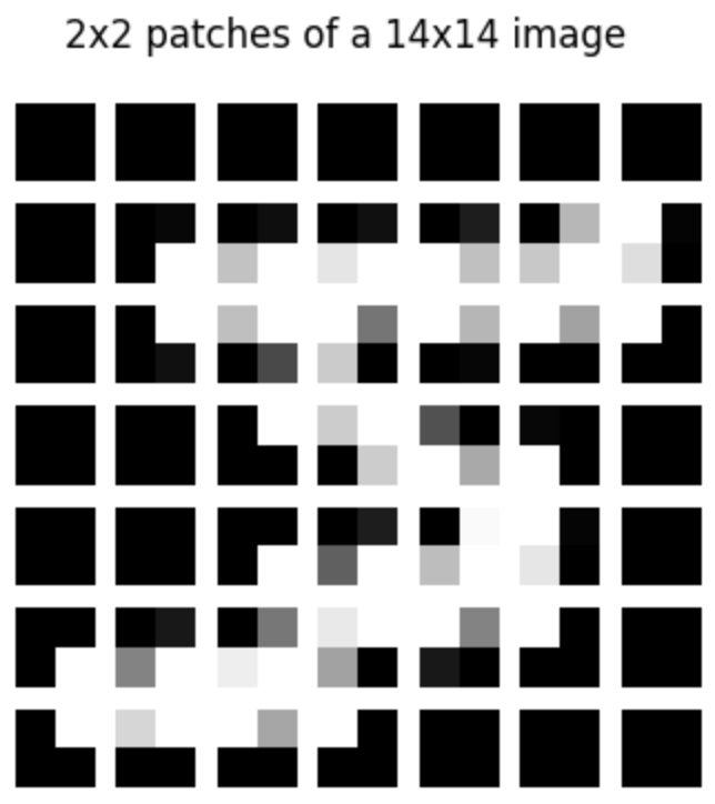
The important thing to notice is that a patch is still an image. Nevertheless, transformer are trained to predict a single token-id belonging to a vocabulary not a grid of pixels

TOKENIZER Therefore, we need a tokenizer that map each possible patch to an integer id. For this reason, we can see that the size of the vocabulary of id \(V\) will grow exponentially with the number of possible value of each pixel and the size of the patch:

If we allow a pixel \(x\) to be in \(\{1,...,255\}\) and we use patch of \(2 \times 2\) then we will have \(\#V = 255^4 = 4.2 \times 10^9\).

BINARIZATON For this reason we see that we are forced to binarize the pixel in black and white. Now we have \(\# V = 2^4 = 16\) id.

INTEGER-ID Once they are binarised, we can simply define a tokenizer map

So for example:

1.2 Transformer-Block

1.2.1 Forward Pass (Pre/Post)

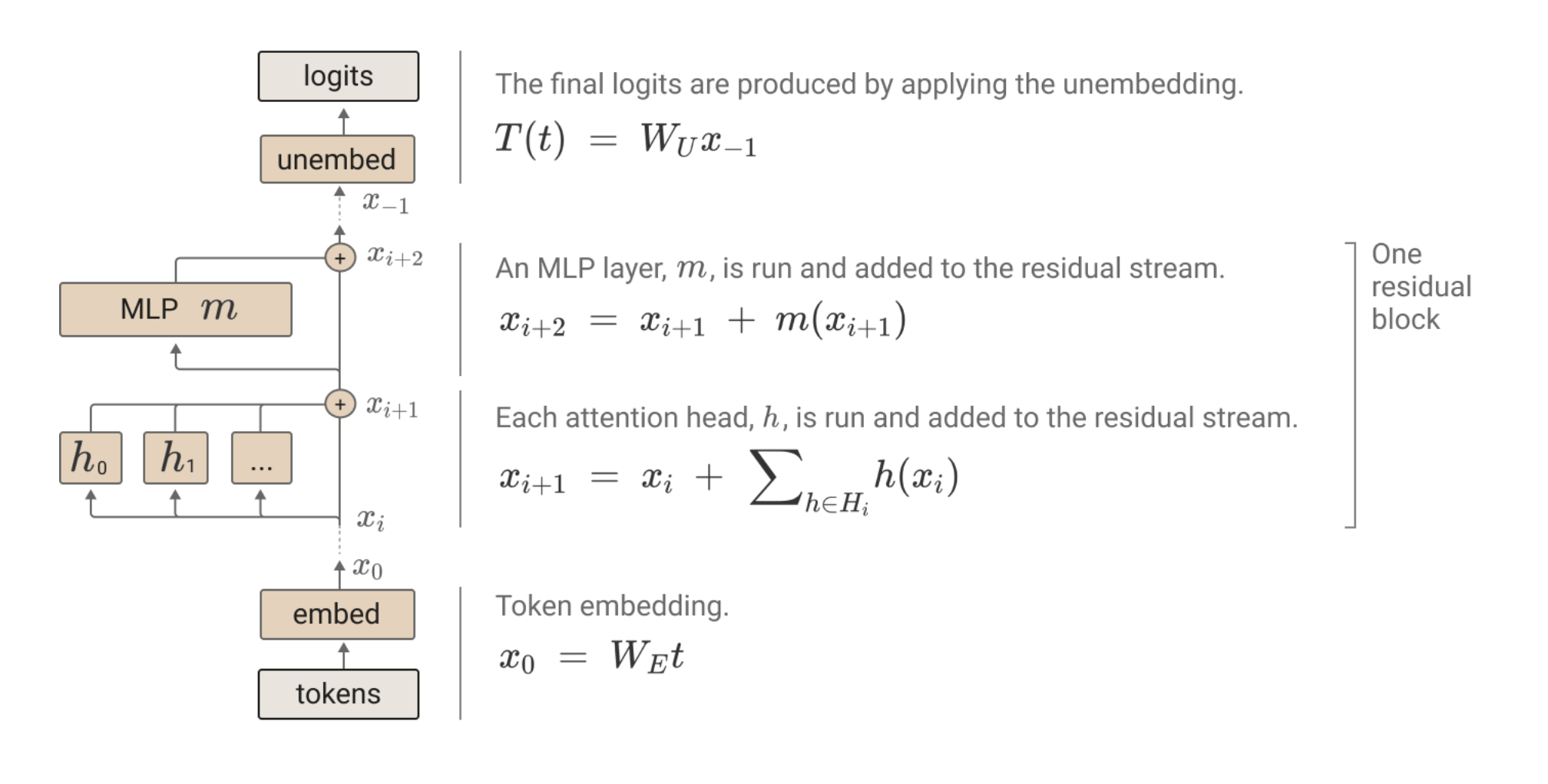
READ AND WRITE ON RESIDUALS Information is read and written from the residual stream by Attention Layers and MLPs:

Where \(t\) is the number of tokens and \(d\) is the hidden dimension. Therefore, each row is an vector representation of a token.

POST-LAYER-NORM ARCHITECTURE Information is written normalised on the residual stream. Pass:

PRE-LAYER-NORM ARCHITECTURE Information is read normalised on the residual stream. Pass:

1.2.2 Multi-Head Attention

FLOW OF COMPUTATION The flow of the attention mechanism is the following:

1. linear projection of input \(X \in R^{t \times d}\) in \(Q,K,V \in R^{t \times d}\). Mathematicaly: \(Q = X W_Q, \quad K = X W_K, \quad V = X W_V\)

   Instead, it can be done programatically by:

    # inside the init of the class
    self.w_Q = nn.Linear(model_dim, model_dim, bias = False)
    self.w_K = nn.Linear(model_dim, model_dim, bias = False)
    self.w_V = nn.Linear(model_dim, model_dim, bias = False)
   
    # inside the forward: b x t x d -> b x t x d
    q = self.w_Q(x)
    k = self.w_K(x)
    v = self.w_V(x)
   

2. creation of \(n\) attention head of dimension \(h = d // n\) such that \(Q_i, K_i, V_i \in R^{t \times h}\). Programtically this is done via einops.rearrange

    # inside the forward: b x t x d -> # b x n x t x h
    k = rearrange(k, "b t (n h) -> b n t h", n = self.n, h = self.h) 
    q = rearrange(q, "b t (n h) -> b n t h", n = self.n, h = self.h) 
    v = rearrange(v, "b t (n h) -> b n t h", n = self.n, h = self.h) 
    # alternatively: k.view(b, t, n, h).permute(0, 3, 1, 2)
   

3. creation of row similarity database between rows of \(Q_i\) and \(K_i\) → \(Q_iK_i^T\). Program:

    # compute similarity scores: b x n x t x h -> b x n x t x t
    s = einsum(q,k, "b n t1 d, b n t2 d -> b n t1 t2")
   
    # alternatively: q @ k.pemute(0,1,3,2)
   

4. normalize, apply masking and turn to probability row via softmax $$ S_i = \text{softmax}!\left(\frac{Q_iK_i^\top}{\sqrt{d_h}} + \text{mask}\right)

   $$

   To implement this:

    # apply the normalization
    s = s / np.sqrt(self.h)
    # apply the mask 
    s = s + mask
    # apply softmax
    s = F.softmax(s, dim = -1) 
   

5. get new matrix as with \(t\) rows (one for token) where each row is the convex combination of the row of \(V\) via the probability distribution obtained before \(S_iV_i\)

    # b x n x t x h
    weighted_mean = einsum(s,v, "b n t1 t2, b n t2 h -> b n t1 h") 
   
    # alternatively: s @ v
   

6. Concatenate the results and project it back with

    weighted_mean = rearrange(weighted_mean, " b n t h -> b t (n h)")
    mha = self.w_O(weighted_mean) 
    # equivalently weighted_mean.permute(0,2,1).view(b,n, -1)
   

FORMULA ATTENTION This brings to the following formula for general attention:

FORMULA MHA And to its generalization to multihead attention

1.2.3 Layer Norm

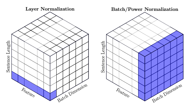
The block computes variance and expectation of \(X \in R^{t \times d}\) along d, so each token as its own information and is not used for other like in batch-norm:

Visually they compare like this:

Code-wise just init two parameter for bias and scaling and then compute the unbiased var and the mean

class LayerNorm(nn.Module):

    def __init__(self, dim: int, eps = 1e-05, bias = True):

        super().__init__()
        # storing the dimension
        self.dim = dim
        self.eps = eps

        # creating two parameter
        self.gamma = nn.Parameter(torch.ones(dim))
        self.bias = nn.Parameter(torch.zeros(dim))
    
    def forward(self, x):

        # aggregates
        mean = x.mean(dim = -1, keepdim = True)
        var = x.var(dim = -1, keepdim = True, unbiased=False)
        # scale
        x = (x-mean) / torch.sqrt(var+self.eps)
        # apply parameter
        return x*self.gamma + self.bias

1.2.4 MLP

Applies two linear layers with an activation in between:

It uses an higher dimensional projection dimension (so W₁ has more rows than column)

class MLP(nn.Module):

    def __init__(self, input_dim, hidden_dim, output_dim):
        """
        input_dim: dimension of input features
        hidden_dim: dimension of hidden layer
        output_dim: dimension of output features
        """
        super().__init__()
        self.linear1 = nn.Linear(input_dim, hidden_dim) # bias default true
        self.activation = nn.GELU()
        self.linear2 = nn.Linear(hidden_dim, output_dim) # bias default true


    def forward(self, x):
        """
        x: input tensor of shape (..., input_dim)
        returns: output tensor of shape (..., output_dim)
        """
        x = self.linear1(x)
        x = self.activation(x)
        x = self.linear2(x)

        return x 

1.3 Autoregressive Transformer

1.3.1 Forward Pass

A visualization of the forward pass is here

Otherwise, check it here:

# in the init 
self.blocks = nn.ModuleList([ TransformerBlock(self.d_model, self.n_heads, self.d_ff, False) for _ in range(self.n_layers)])
# forward
def forward(self, x):
		# positional and embedding
    x = self.pos_embedding(x) + self.embedding(x)
    # forward pass 
    for layer in self.blocks:
        x = layer(x, self_mask = mask)
    # unembedding
    return self.projection(self.norm(x))

1.3.2 Token Embeddings

Transforming the discrete tokens (integers id) into a sequence of learnable vector representations. Luckily, nn.Embeddings is already implemented:

self.token_embedding = nn.Embedding(vocab_size, model_dim)

1.3.3 Positional Embeddings

For these you can use, for instance, learnable positional embeddings. You should support a maximal sequence length of max_seq_length. They should be added to the embedded tokens.

# in the init
self.pos_embedding = nn.Embedding(max_seq_length, model_dim)

# to use it we must extract the relative position 
batch_size, seq_length = x.shape
positions = torch.arange(0, seq_length).unsqueeze(0).expand(batch_size, seq_length)

x = torch.tensor([[1], [2], [3]])
x.size()
torch.Size([3, 1])
x.expand(3, 4)
tensor([[ 1,  1,  1,  1],
        [ 2,  2,  2,  2],
        [ 3,  3,  3,  3]])
x.expand(-1, 4)   # -1 means not changing the size of that dimension
tensor([[ 1,  1,  1,  1],
        [ 2,  2,  2,  2],
        [ 3,  3,  3,  3]])

1.3.4 Prediction Head

As easy as it can be:

self.projection = nn.Linear(model_dim, vocab_size, bias=False)

1.3.5 Sampling

Mathematically, is simple: we have a multinomial distribution that assign to each index a given probability and that sums to 1. We must sample. The only trick is to use a temperature parameter. For more details see this chat with gemini:

• temperature to 1 → nothing changes
• temperature > 1 (smoothing)→ shrink everything near 0 (big positive → small positive, big negative → small negative) so probability becomes more mild (convergence to uniform)
• temperature<1 (sharpening)→ makes difference bigger, decreasing the entropy (diverge from uniform) Programatically, we just need to sample with torch.multinomial

@torch.no_grad()
  def sample_next_token(self, x, temperature=1.0):
      """
      x: input tensor of shape (batch_size, seq_length)
      returns: output tensor containing logits of shape (batch_size,)
      """
      logits = self.forward(x) # (batch_size, seq_length, vocab_size)
      probs = F.softmax(logits[:, -1, :]/temperature, dim=-1)
      next_token = torch.multinomial(probs, num_samples=1)[:,0] # clean extradimension
      return next_token

weights = torch.tensor([0, 10, 3, 0], dtype=torch.float) # create a teso
r of weights
torch.multinomial(weights, 2)
tensor([1, 2])
torch.multinomial(weights, 5) # ERROR!
RuntimeError: cannot sample n_sample > prob_dist.size(-1) samples without replacement
torch.multinomial(weights, 4, replacement=True)
tensor([ 2,  1,  1,  1])

2. T5, GPT, and Bert (N6-E6)

Transformer-based architectures have been the foundation of many popular models, such as BERT (encoder-only), T5 (encoder-decoder), and GPT (decoder-only). In this section we will compare them.

2.1 Forward Passes

2.1.1 Common Transformer Block

The base block of the three architecture is the same. Let′s work with a pre-layer block (so read information normalised).

• ENC VS DEC Between encoder and decoder the only difference is the mask we pass for the self attention.
• ENC + DEC In this case we simply add one step to the forward pass where we read the

  def forward(self, x, mask=None, encoder_output=None, cross_mask=None):
        """
        x: input.
        mask: mask for encoder-only or decoder-only structures.
        encoder_output: used in T5, the source of K and V for cross-attention.
        cross_mask: used in T5, the mask for cross-attention.
        """
        x = x + self.self_attn(self.norm1(x),self.norm1(x), mask)
        # ONLY FOR T5
        if self.cross and encoder_output is not None:
            x = x + self.self_attn_cross(self.norm_cross(x), encoder_output, cross_mask)
        x = x + self.ffn(self.norm2(x))
        return x 
  

2.1.2 Different Transformer Passes

While the base block is the same there are some difference in the forward pass of the transformer.

BERT and GPT are as simple as:

embedding(x)+pos(x)-> block(x) n times -> normalized projection.

Programatically they are:

def forward(self, x):
        # compute mask
        mask = causal_mask(X) & pad_mask(x)
        # embedd
        x = self.pos_embedding(x) + self.embedding(x)
        # forward pass 
        for layer in self.blocks:
            x = layer(x, mask, None, None)
        # unembedding
        return self.projection(self.norm(x))

T5 Instead is a bit more convoluted:

def forward(self, x, y):
				# encode it, compute output and mask for cross-attention
        encoder_output, cross_mask = self.encode(x)
        # decode it 
        output = self.decode(y, encoder_output, cross_mask)
        return output

While the encoder is the same as the BERT, the decoder will need cross-attention so is a bit different:

# INSIDE DECODER FORWARD 
for layer in self.blocks:
	x = layer(x, mask, encoder_output, cross_mask)

2.2 Attention

2.2.1 Core Ideas (E6.1)

BERT each layer of the encoder use attention with both \(Q,K,V\) ← \(X_{enc}\) read from the residual stream of the encoder

• Masking is the padding mask for bidirectional attention mechanisms GPT each layer of the decoder use attention with both \(Q,K,V\) ← \(X_{dec}\) read from the residual stream of the decoder

• Masking is the causal masking so that token at position \(t\) from \(V\) is obtained by attending information from \(Q,K\) only from \(\leq t\) T5 there are three type of attention:

• encoder: the encoder has simply BERT encoder attention with pad-masking and \(Q,K,V\) ← \(X_{enc}\)
• decoder: the decoder has two type of attention:
  • decoder has a first attention that is GPT like
  • there is another type of attention at each transformer block, added after the first attention, that is cross-attention.
    • takes as Q←\(X_{dec}\), and \(K,\)V ← \(X_{enc}\).
    • NB: At each transformer-block of the decoder, while \(X_{dec}\) is updated as we proceed along this residual stream, the global information outputed by the encoder \(X_{enc}\) remain the same.
    • cross-attention compute \(Q_{dec}K_{enc}^T\) which means that a row of this matrix, let′s say the third, is how similar is the third of row of \(Q_{dec}\), so decoder third token hidden representation, to each row of \(K_{enc}\) so each input of the encoder.
      • So when we right multiply \(SV_{enc}\) then the output of cross attention, e.g. the 5th row, is the weighted mean of the encodeder hidden representations based on how similar they are to the 5th token/row of \(Q_{dec}\)

        2.2.2 Attention Implementation

You can implement all these type of attention with the same code we outlined above form MHA. Indeed, the differences between these types of attention depends only on the:

• D1: input representation (is Q coming from the same place of K,V?)
  • used to distinguish between cross and self-attention
• D2: attention mask
  • used to distinguish causal vs non-causal attention

The mask was compute outside and passed to the attention, so D2 is already implemented. The only things we need to do is D1

# OLD IMPLEMENTATION
def forward(self, x,  mask=None):
	"""
	input arg becomes q_input, kv_input.
	if self-attention q_input == kv_input
	"""
	q = self.w_Q(x)
	k = self.w_K(x)
	v = self.w_V(x)
		
	# same
	...
		
# NEW MECHANISM
def forward(self, q_input, kv_input, mask=None):
	"""
	input arg becomes q_input, kv_input.
	if self-attention q_input == kv_input
	"""
	# projections are modified to have D1
	q = self.w_Q(q_input) # b x t x d
	k = self.w_K(kv_input)
	v = self.w_V(kv_input)
	
	# same
	...

2.3 Masking

2.3.1 Pad Mask

GOAL Blocking attention row-similarity database to look at PAD tokens as contain no info

We can do this with this code

def pad_mask(x, pad=Tokenizer["PAD"]):
    """
    x: b x t
    output -> 1 x 1 
    """
    return (x != pad).unsqueeze(1).unsqueeze(2)

# 1. fake input 
x = torch.arange(0,9).reshape(3,3)+ 31992
# output
tensor([[31992, 31993, 31994],
        [31995, 31996, 31997],
        [31998, 31999, 32000]])

# 2. apply mask 
pad = 32000
(x != pad)
# output
tensor([[ True,  True,  True],
        [ True,  True,  True],
        [ True,  True, False]])
        

2.3.2 Causal Masks

GOAL Blocking attention row-similarity database to look at future tokens as it creates label leaking

IDEA The idea is that we want to mask the matrix \(QK^T\) such that for a given row, the right position after the diagonal count are False. It is easier to see:

True, False, False
True, True, False
True, True, True

We can do this with this code:

def causal_mask(t):
    """Causal mask for decoders."""
    return torch.tril(torch.ones(t, t, dtype=torch.bool)).view(1, 1, t, t)

# 1. get a bool matrix tokens x tokens
t = 3
bool_matrix = torch.ones(t, t, dtype=torch.bool)
# output 
tensor([[True, True, True],
        [True, True, True],
        [True, True, True]])
        
# 2. get a upper triangular matrix
mask = torch.tril(bool_matrix)
# output
tensor([[ True, False, False],
        [ True,  True, False],
        [ True,  True,  True]])

2.4 Positional Encoding

2.4.1 Positional Encoders

TYPES Broadly, positional encodings fall into two families: absolute and relative.

ABSOLUTE ENCODERS Attach an absolute position signal to each token independently. Examples are:

1. learned encoding for a max_context window

2. sinusoidal encoding, which use deterministic sine/cosine features without learned parameters (attach to each index of the hidden dimension a cos/sin function with a given frequency and take as input the token position) RELATIVE ENCODERS inject information about the offset between a query at position i and a key at position j inside the attention module, so that the attention score depends on (j − i). So, if two tokens differ for 5 positions, the model will not have a distinct signal if they are the 1 and 6 or the 13024 and the 13029. The important property is that they are applied to attention logits

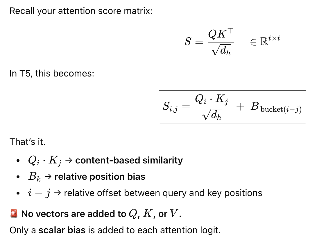
3. T5 original encoding is not done via x = embedding(x)+encoding(x) at the beginning of the forward pass. Instead, it computes a scalar values for each \((i-j)\) and store it to add it to the attention logits
   more details

   

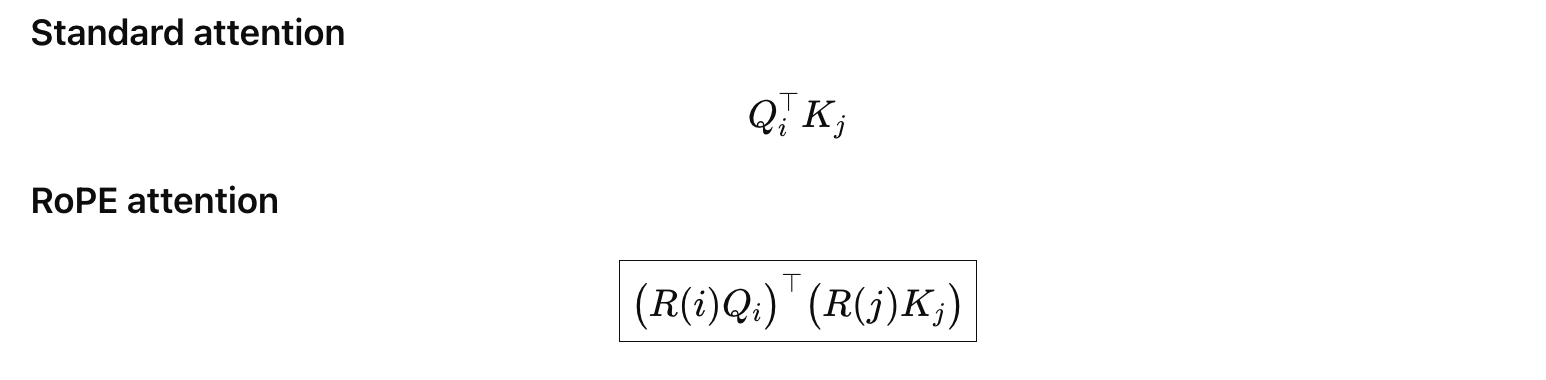
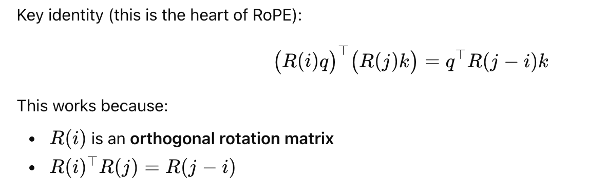
4. ROPE it rotates the Q and K attention logits by applying a rotation matrix R so that in the attention computation of the score \(QK^T\) the dot product for two rows corresponging to two different positions depends only on the relative difference in position \((i-j)\) rather than the absolute position \(i,j\)
   more details

   

   

NO EXPLICIT ENCODING Recently, NoPE (No explicit Positional Encoding) is also being explored. In the decoder-only models, one can omit explicit positional embeddings and rely on the causal mask to indicate positions

PROS AND CONS

• Absolute Learned positional encodings are simple but struggle with length extrapolation (train short, test long). For example, learned absolute embeddings cannot extend to lengths beyond the training range, because positions unseen during training have no learned parameters.
• Relative positional encodings typically handle length generalization better and are common in modern LLMs.
• NoPE is extremely simple and parameter-free; it relies only on the causal mask for an implicit positional bias and can yield the best length generalization. However, training NoPE models from scratch can be difficult.

2.5 Tokenizer

• standard extra token of the three architectures

2.6 Losses

2.6.4 Torch Implementation

In practice all loses are implemented in the same way in torch:

# logits and labels extracted from forward pass and dataloader
logits.shape == (batch_size, seq_len, vocab_size)
y.shape == (batch_size, seq_len)

# turning stackin batch on the seq_len dimension 
y_stacked = y.view(-1) # (batch_size * seq_len)
logit_stacked = logits.view(-1, vocab_size)# (batch_size * seq_len, vocab_size)

# compute cross-entropy and ignore -100, we set to those mask
loss = F.cross_entropy(logit_stacked,y_stacked, ignore_index=-100)

Open Questions

• • What will happen if you increase or decrease the p_mask variable in BERT and T5 training?
• • If keep increasing the sequence length in the Config in model.py, do you observe any memory issues in training the models? Do you know why?

E5: Attention Transformers and Tokenisation

RAM Systems

Floating Point Operations

Count the raw number of arithmetic operations (sum, multiplication …) required, ignoring parallelism or hardware specifics.

• Vector Addition (\(v + v\)): Given \(v \in \mathbb{R}^d\). Require \(d\) additions/FLOPs.
• Scalar Multiplication (\(c \cdot v\)): Given \(v \in \mathbb{R}^d\). Requires \(d\) multiplications/FLOPs.

Cost of Vector Dot Product

• \(v^T w\): Given \(v, w \in \mathbb{R}^d\). Requires \(d\) multiplications and \(d-1\) additions. Total: \(\approx 2d\) FLOPs.

Cost of Matrix-Vector Multiplication

• \(Av\): Given matrix \(A \in \mathbb{R}^{b \times d}\) and vector \(v \in \mathbb{R}^d\) The result is a vector in \(\mathbb{R}^b\). We perform \(b\) dot products, each involving a vector of size \(d\). Cost per dot product \(\approx 2d\). Total: \(2bd\) FLOPs.

Matrix-Matrix Multiplication

• \(AB\): Given matrices \(A \in \mathbb{R}^{b \times d}\) and \(B \in \mathbb{R}^{d \times c}\). The result is a \(b \times c\) matrix. We must compute \(b \times c\) individual elements. Each element is the result of a dot product of size \(d\) (row of \(A\) dotted with column of \(B\)). Total: \((bc) \times 2d = 2bdc\) FLOPs.
• In the same scenario, given \(A, B\) and \(k \in R^{c}\), then \(ABk\) requires \(2bd + 2bc\) FLOPs

The Forward Pass of Attention Models

Number of Learnable Parameters of Attention

We are estimating the storage footprint of a single multi-head attention block (ignoring biases)

• Key Components:
  • Input Projections: We have three distinct weight matrices for the Query (\(W^Q\)), Key (\(W^K\)), and Value (\(W^V\)). Each has a shape of \(d_{model} \times d_{model}\).
  • Output Projection: After the heads are concatenated, there is one final linear projection \(W^O\), also with shape \(d_{model} \times d_{model}\)
  • Total Parameters: \(4 d_{model}^2 = O(d_{model}^2)\)
• Note: The parameter count is independent of the number of heads ($h$) because the splitting into heads happens via reshaping the computed tensors, not by changing the size of the initial weight matrices

FLOPs for Attention Pass

input tensor \((1, n, d_{model})\).

Step A: Q, K, V Projections (Linear Layers)

• Operation: Three matrix multiplications of \((n \times d_{model}) \times (d_{model} \times d_{model})\)
• Calculation: \(3 \times (2 \cdot n \cdot d_{model} \cdot d_{model})\)
• Cost: \(6 n d_{model}^2\)

Step B: Attention Scores (\(Q K^T\))

• Operation: For each head, multiply \((n \times d_k)\) by \((d_k \times n)\).
• Calculation: \(h \times (2 \cdot n \cdot d_k \cdot n) = 2 n^2 (h \cdot d_k)\).
• Cost: \(2 n^2 d_{model}\).

Step C: Scaling & Softmax

• Operation: Element-wise scaling by \(1/\sqrt{d_k}\) and softmax exponentials/divisions on scores \((n, n, h)\)
• Cost: \(O(n^2 h)\)

Step D: Weighted Sum (\(Attention \cdot V\))

• Operation: For each head, multiply Softmax output \((n \times n)\) by \(V\) \((n \times d_k)\).
• Calculation: \(h \times (2 \cdot n \cdot n \cdot d_k) = 2 n^2 (h \cdot d_k)\).
• Cost: \(2 n^2 d_{model}\).

Step E: Output Projection

• Operation: One matrix multiplication of \((n \times d_{model}) \times (d_{model} \times d_{model})\)
• Calculation: \(1 \times (2 \cdot n \cdot d_{model} \cdot d_{model})\)
• Cost: \(2 n d_{model}^2\)

Total FLOPs for foward pass of attention block

• Summing all components: \(\text{Total} \approx 8 n d_{model}^2 + 4 n^2 d_{model} + O(n^2 h)\)
• In paractice \(O(n^2 h)\) is dominated by the rest

Efficiency Bottleneck

• high number of heads ⇒ slow down scaling + softmax as \(O(n^2 h)\)
• high latent dimentions ⇒ slow down projection as \(O(n d_{model}^2)\)
• high numner of tokens ⇒ slow down \(QKV\) circuits as \(O(n^2 d_{model})\)

E6: Attention Transformers and Tokenisation

BERT, T5, and GPT models

Model Architectures & Attention Flows

The key difference lies in Masking and where the Query/Key/Value vectors come from.

• Encoder-Only (BERT) ◦ Goal: Learn contextual representations of the whole input ◦ Attention: Uses Self-Attention where Q, K, V all come from the encoder hidden states ◦ Masking: Bidirectional. Every token attends to every other token (no mask)
• Decoder-Only (GPT)
  • Goal: Learn left-to-right generative modelling
  • Attention: Uses Self-Attention where Q, K, V come from the decoder hidden states
  • Masking: Causal (Upper-Triangular). At position t can only attend to positions \(\le t\)
• Encoder-Decoder (T5)
  • Goal: Separate source encoding from target generation (sequence-to-sequence)
  • Attention Types:
    1. Encoder Self-Attention: Bidirectional (like BERT)
    2. Decoder Self-Attention: Causal (like GPT)
    3. Cross-Attention: The Decoder supplies the Queries while the Encoder supplies the Keys and Values. This allows the decoder to “look back” at the whole input

Positional Encodings

• Absolute Encoding (BERT & GPT)
  • Mechanism: A specific vector is learned for each position, and added to the token embedding
  • Limitation: It struggles with Length Extrapolation. If trained on 512 tokens, the model has no parameter for position 51312.
• Relative Encoding (T5)
  • Mechanism: Instead of input embeddings, T5 adds a learnable bias directly to the attention logits (scores) based on the offset (i-j) between tokens
    • maintains separate learned bias tables for each of its three attention types
  • Bucketing: Distances are “bucketed” (nearby positions are distinct; far positions are grouped logarithmically) to handle long sequences efficiently
  • Advantage: Generalizes better to sequence lengths unseen during training
  • How it works: Define one parameter per bucket and simply add it to the attention \(e_{i,j} = \frac{Q_i K_j^T}{\sqrt{d_k}} + \beta_{(i-j)}\)
• Modern Alternatives
  • RoPE (Rotary): Rotates query/key vectors so their dot product reflects their relative distance. Standard in Llama/Mistral
  • NoPE: Uses no explicit encoding; relies entirely on the causal mask to provide position information. Difficult to train from scratch

Training pipelines and objectives

• BERT: Masked Language Modeling (MLM)
  • Method: Randomly selects 15% of tokens. Replaces them with [MASK] (80%), random token (10%), or keeps original (10%)18.
  • Objective: Predict the original token for the masked positions only based on context \(\mathcal{L}_{MLM} = -\sum_{i \in M} \log p_{\theta}(x_i \vert x_{\setminus M})\)
• GPT: Autoregressive (Causal) Modeling
  • Method: Predicts the next token in the sequence given all previous tokens
  • Objective: Standard left-to-right likelihood maximization \(\mathcal{L}_{AR} = -\sum_{i=1}^{t} \log p_{\theta}(x_i \vert x_{<i})\)
• T5: Span-Corruption
  • Method: Replaces contiguous spans of text in the encoder input with sentinel tokens (e.g., <extra_id_0>)
  • Target: The decoder must generate only the dropped-out spans, separated by the sentinels \(\mathcal{L}_{T5} = -\sum_{s=1}^{ \vert y \vert } \log p_{\theta}(y_s \vert y_{<s}, \text{Enc}(x^{masked}))\)

A Mental Model for GPU memory and its management

• GPU memory is hierarchical
  • We have big slow (global) memory (DRAM), and small fast (shared) memory (SRAM). To perform computations, data has to be moved from the slow memory to the fast memory
  • There are two possible memory bottlenecks: -storage: when global memory is not large enough -memory traffic: when moving data from global to shared memory is slow
• To analyse whether an operation is “Compute-Bound” (limited by calculation speed) or “Memory-Bound” (limited by data transfer speed). We measure this using Arithmetic Intensity (AI), defined as the ratio of FLOPs performed to bytes moved
  • \[AI = \frac{\text{Total FLOPs}}{\text{Total Bytes Accessed}}\]
    • If the AI is low, the GPU spends more time waiting for data than calculating (Memory-Bound). If AI is high, it spends more time calculating (Compute-Bound).
      • we want it to be compute bound so we use the most of the computational power
  • We can compare it with the detailed statistics of GPUs. Let the critical arithmetic intensity (ridge point) be \(I^∗\) = Peak FLOPs/Peak memory bandwidth. For A100 80GB (HBM2e ≈ 2.0 TB/s, BF16 Tensor Core ≈ 312 TFLOPs), \(I^∗\) ≈312/2.0≈ 156 FLOPs/Byte. For H100 SXM (HBM3 ≈ 3.35 TB/s, BF16 Tensor Core ≈ 989 TFLOPs), \(I^∗\) ≈989/3.35≈295 FLOPs/Byte
    • if an operation’s AI exceed the \(I^*\) it is Compute bound; if it is below it is Memory bound

Memory traffic

We now analyse the memory traffic for training/prefilling and decoding modes.

• Linear Projections
  • Scenario: Input \(X\) ( \(b \times t \times d\) ) multiplied by Weights \(W\) ( \(d \times d\) ).
  • Data Moved (Bytes): We must read \(X\), read \(W\), and write Output \(Y\) ( \(b \times t \times d\) ) + ( \(d \times d\) ) + ( \(b \times t \times d\) ) = ( \(2btd\) + \(d^2\) ) \(\times s\) (where \(s\) is bytes per element, e.g., 2 for bf16)
  • Operations done (FLOPS) \(\approx 2btd^2\)
  • \[AI_{lin} \approx \frac{2btd^2}{(2btd + d^2)s}\]
  • Training (\(bt \gg d\)): The \(2btd\) term dominates the denominator. The ratio simplifies to \(\approx d/s\). For a standard model (\(d=4096, s=2\)), AI is \(\approx 2048\) which is Compute-Bound.
  • Decoding (\(t=1\) ): The data movement for weights (\(d^2\)) becomes significant compared to the small amount of computation. The AI drops to \(\approx 2b/s\), making it Memory-Bound
• Scaled Dot-Product Attention
  • Core attention mechanism: \(Softmax(QK^T)V\)
  • Scenario: Full score matrix \(S = Softmax(QK^T)\) of size ( \(b \times a \times t \times t\) ), where \(a\) is the number of heads.
  • Data Moved (Bytes): read Q + read K + write S + read S + read V + write O Reading Q, K, V, O is small ( \(btd\) each), but reading/writing the massive score matrix \(S\) ( \(bat^2\) ) is huge: \(\text{Bytes} \approx (4btd + 2bat^2)s\)
  • Compute (FLOPs) \(\approx 4bt^2d\)
  • \[AI_{attn} \approx \frac{2td}{s(2d + at)}\]
  • Memory-Bound Nature: When \(t ≫ 2d/a\) (often since \(d/a = h \in \{64,128\}\)) \(AI_{attn} \approx \frac{2td}{s(2d + at)} \approx \frac{2d}{sa}\) which is quite small, hence, Memory bound Decoding: we must load the entire KV cache for every new token generated. This creates massive memory traffic, hence, Memory bound
    • approaches like FlashAttention-style kernels improve

Memory storage

We now look at whether the GPU has enough DRAM (e.g., 80GB on an A100) to hold the necessary data

• Decoding (KV cache bottleneck)
  • We must store the Key and Value matrices for every previous token to avoid re-computing them at every step To cache a batch \(b\) of sequences with length \(t\), across all layers \(L\):

  \(\text{Total Bytes} = L \times b \times (2 \cdot d \cdot t) \times s\) (Where 2 accounts for K and V, and \(s\) is bytes per element, usually 2)

  For a 7B model (\(L=32, d=4096\)) on an A100 M=80GB GPU: If the sequence length is 4096, the memory is so full that the maximum batch size is only \(\approx\) 40.

  • In practice, because model weights also take space (7B weights in bf16 ≈ 14 GiB), it is closer to 28-32 Note: Still to use the cached K and V we still have to load them to fast memory which slows down the decoding more
• Training: The Optimizer State Bottleneck
  • Training runs out of memory faster than inference because of the Optimizer States (like Adam), which are often stored in higher precision (FP32)
  • Rule of thumb: Memory for every parameter in the model: \(\text{Bytes per Param} \approx \underbrace{2}_{\text{weight}} + \underbrace{2}_{\text{gradient}} + \underbrace{4}_{\text{momentum } m} + \underbrace{4}_{\text{variance } v} = \mathbf{12}\) There is also an optional fp32 master copy (optional +4)
  • Example: A 7B parameter model requires \(\approx\) 84GB (105GB if we keep a master copy of the parameters) just for these states, ignoring activations needed for backprop

  This forces the use of Sharding: splitting the model/states across multiple GPUs, e.g., ZeRO