Notes on Vision Models
A. MAE, and iBOT (E7)
Our focus is on a trio of seminal self-supervised learning methods for computer vision:
- Masked Autoencoders (MAE),
- Image BERT Pre-Training with Online Tokenizer (iBOT)
- knowledge DIstillation with NO labels (DINO).
1.0 Masked Autoencoders (MAE)
CORE IDEA MAE Masked Autoencoders (MAE) core concept is intuitive: the model learns rich visual representations by reconstructing masked or missing portions of an input image.
1.1 Core Architecture and Pre-training Mechanism
The MAE pre-training process, as illustrated in the architectural overview, is notable for its efficiency and elegant design. The procedure unfolds in several key steps:
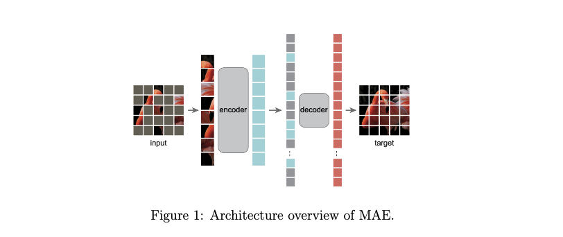
- Patching and Masking: An input image is first divided into a grid of non-overlapping patches. A large, random subset of these patches (e.g., 75%) is then masked, making them invisible to the encoder.
- Encoding Visible Patches: The MAE encoder, a standard Vision Transformer, processes only the small subset of visible patches. This is a critical design choice for efficiency.
- Introducing Mask Tokens: After the visible patches have been encoded, learnable “mask tokens” are introduced to represent the positions of the patches that were originally masked.
- Decoding and Reconstruction: A small, lightweight decoder takes the full sequence of encoded patches and mask tokens as input. Its sole task is to reconstruct the original, uncorrupted image in pixel space from this limited information.
COMPUTATIONAL EFFICIENCY This asymmetric encoder-decoder design is the cornerstone of MAE’s computational efficiency. By applying the large, computationally expensive encoder to only a fraction of the input (e.g., 25%), MAE dramatically reduces training time and memory requirements.
1.2 Adapting Masked Modeling from Language (BERT) to Vision (MAE)
CHALLENGE OF MAE TEXT → VISION The success of masked modeling in natural language processing (NLP) with models like BERT inspired MAE, but these are challenges:
- Information Redundancy: Images exhibit high spatial redundancy; neighboring patches often contain very similar information.
- SOLUTION → To create a challenging learning task, MAE must use a very high masking ratio (e.g., 75%). In text, information is denser and a lower masking ratio (e.g., 15% in BERT) is sufficient.
- Tokenization: Language has a natural, discrete unit: the word or sub-word token. Images are continuous signals.
- SOLUTION → MAE must therefore make an architectural decision to segment an image into a grid of patches, creating a set of “visual tokens.”
- Semantic Density: A single word token in text typically carries a concentrated semantic meaning. An individual image patch, however, may contain very little semantic information on its own, forcing the model to learn spatial relationships and global context.
- Reconstruction Target: BERT predicts discrete tokens from a finite vocabulary. MAE’s decoder reconstructs continuous pixel values → output space fundamentally different
- SOLUTION → use different loss such as MSE
- Computational Efficiency: The quadratic complexity of transformers is more problematic for images, which typically yield a much larger number of tokens (patches) than a sentence.
- SOLUTION → MAE’s asymmetric design has big encoder that process few tokens and small decoder that process everything
1.3 Analysis of MAE’s Pre-training Effectiveness
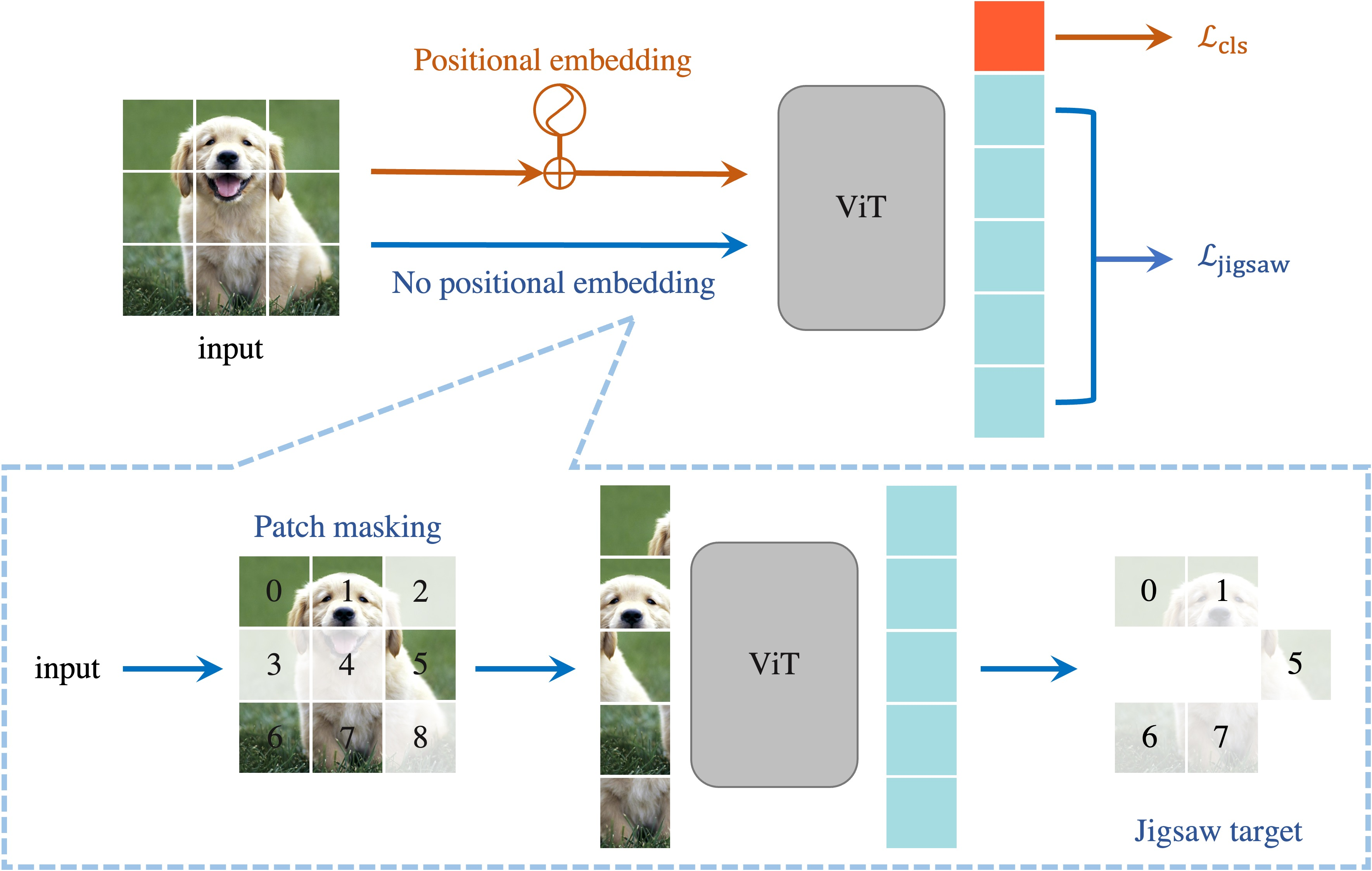
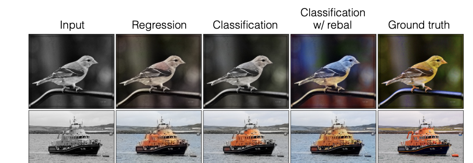
OLD LOSS Prior to MAE, several other self-supervised pretext tasks for vision were proposed:
- jigsaw puzzles → predict the right position of the patch
- in-coloring → (predicting color from a grayscale image)
ADVANTAGE OF MAE . The MAE framework ultimately prevailed due to a combination of factors:
- simplicity → The pixel-reconstruction objective is straightforward to implement
- scalability → computational efficiency of the asymmetric encoder-decoder design, allows MAE to scale to enormous models and datasets.
1.4 A Deeper Look at Masking Strategies
MAE MASKING TYPES we say that MAE reconstruct mask but how should we mask? These are three possible type coherent with masking
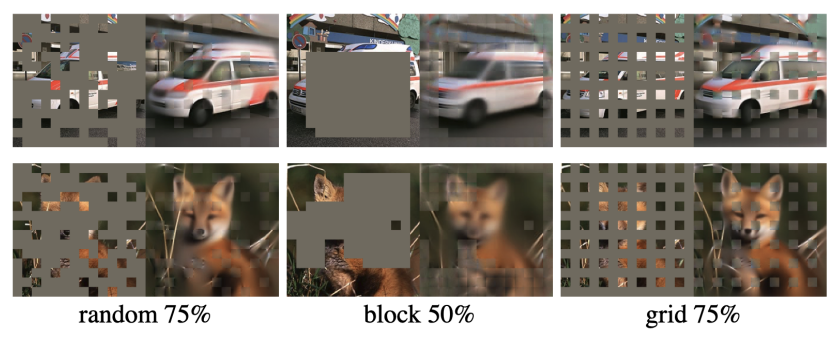
- Random Masking: This strategy proved to be the most effective.
- By removing patches without any discernible spatial structure → prevents the model from “cheating” by exploiting local continuity or predictable patterns.
- This forces the development of a global contextual understanding and the learning of holistic, robust representations.
- Block-wise Masking: This approach removes contiguous rectangular regions
- While this may encourage object-level reasoning
- the task is generally easier because the predictable boundaries and larger areas of intact local context provide stronger clues for reconstruction.
- Grid-based Masking: This strategy maintains a uniform spatial sampling of visible patches
- The regular intervals make reconstruction easier → the model can often rely on simple spatial interpolation from neighboring visible patches
random masking is the best one + mask 75% not 15% as in text
2.0 Information-Theoretic Rationale for Optimal Masking Ratios (TODO)
A central question in masked modeling is why the optimal masking ratio differs so dramatically between text (BERT at ~15%) and images (MAE at ~75%). The answer lies in the fundamental structure of the data itself. This section provides a formal, information-theoretic argument using the concepts of mutual information and entropy to explain this critical difference.
2.1 Mutual Information in Text Sequences
For a text sequence, we can quantify the amount of information the visible tokens (xv) provide about the masked tokens (xm) using mutual information:
I(xm;xv) = H(xm) − H(xm|xv)
Here, H(xm) is the entropy (uncertainty) of the masked tokens, and H(xm|xv) is the conditional entropy (the remaining uncertainty given the visible tokens).
- The entropy of
mmasked tokens, each from a vocabulary of sizeV, can be approximated as: \(H(xm) ≈ m log V\)- The context from visible tokens reduces this uncertainty. We can model this with an “effective vocabulary size”
Veff(r), which represents the plausible tokens given the context. The conditional entropy is thus:
- The context from visible tokens reduces this uncertainty. We can model this with an “effective vocabulary size”
This gives us the final expression for mutual information in text:
I(xm;xv) = m log(V / Veff(r))
For text, this mutual information decays rapidly as the masking ratio r increases. Text has a 1D sequential structure where information flow is highly dependent on adjacent tokens. Masking even a few words can break this chain in multiple places, severely shrinking the contextual window and making prediction difficult. As more context is removed, Veff(r) quickly approaches the full vocabulary size V, causing the mutual information to plummet towards zero. For example, predicting “sat” in “The cat __ on the mat” is easy, but becomes nearly impossible with a 50% masking ratio in “The __ __ on the __.”
2.2 Mutual Information in Image Patches
For images, we use the analogous concept of differential entropy for continuous data:
I(pm;pv) = h(pm) − h(pm|pv)
In stark contrast to text, the mutual information in images decays slowly as the masking ratio r increases. This resilience is due to several properties of visual data:
- High Spatial Redundancy: Neighboring patches are highly correlated.
- 2D Connectivity: Each patch is surrounded by up to 8 neighbors, compared to only 2 for a word in a sequence. This creates multiple, redundant information pathways. Even if some neighbors are masked, others can provide context.
This property can be analogized to a Markov Random Field (MRF), where a patch is conditionally independent of the rest of the image given its immediate neighbors.
- Because of the dense 2D connectivity, context is preserved far more effectively than in a 1D text sequence.
- Consequently, the difficulty of the prediction task scales differently. At low masking ratios, reconstruction can be solved with simple low-level texture interpolation from neighbors.
- However, at a high masking ratio like MAE’s 75%, the gaps are too large for local interpolation. The model is forced to develop a high-level semantic understanding of objects, shapes, and scenes to infer the missing content, leading to the learning of more powerful representations.
2.3 Mathematical Derivation of Optimal Ratios
The goal of the pre-training task is to find a masking ratio r that maximizes the learning objective. This objective can be modeled as a trade-off between the difficulty of the task (how much information is available) and the strength of the training signal (how much the model has to predict).
L(r) = I(r) · r where I(r) is the mutual information (task solvability) and r is the masking ratio (training signal).
We can model the information decay as an exponential function I(r) = I0 * e^(−λr), where λ is the decay rate. Text has a high decay rate (λtext) and images have a low one (λimages). The learning objective becomes:
L(r) = (I0 * e^(−λr)) · r
To find the optimal masking ratio r*, we take the derivative of L(r) with respect to r and set it to zero:
dL/dr = I0 * e^(−λr) * [1 − λr] = 0
Since I0 and e^(−λr) are always positive, the expression is zero only when 1 − λr = 0. This gives us the optimal ratio:
r* = 1/λ
This elegant result provides our proof. We know from the structural properties of text and images that information decays much faster in text. Therefore, λtext > λimages. Taking the reciprocal of this inequality reverses its direction:
r*text = 1/λtext < 1/λimages = r*images
This formally demonstrates that the optimal masking ratio for text must be lower than for images. A numerical verification using the empirical values (r*text ≈ 0.15 and r*images ≈ 0.75) confirms this:
λtext ≈ 1 / 0.15 ≈ 6.67 λimages ≈ 1 / 0.75 ≈ 1.33
The information decay rate is over 5 times higher for text, consistent with the fundamental difference in data structure.
Having explored the reconstruction-based approach of MAE, we now transition to iBOT, which combines reconstruction with a self-distillation framework.
3.0 iBOT: Fusing Masked Modeling with Self-Distillation
CORE IDEA iBOT (Image BERT Pre-Training with Online Tokenizer) represents a sophisticated evolution in self-supervised learning. Its core innovation is the synergistic combination of two powerful paradigms: the masked prediction task, characteristic of models like BERT and MAE, and the student-teacher self-distillation framework, seen in models like BYOL and DINO. This hybrid approach allows iBOT to learn both fine-grained local features and high-level semantic representations simultaneously.
3.1 Core Architecture and Training Methodology
ARCHITECTURE The iBOT architecture is built around a student-teacher framework.
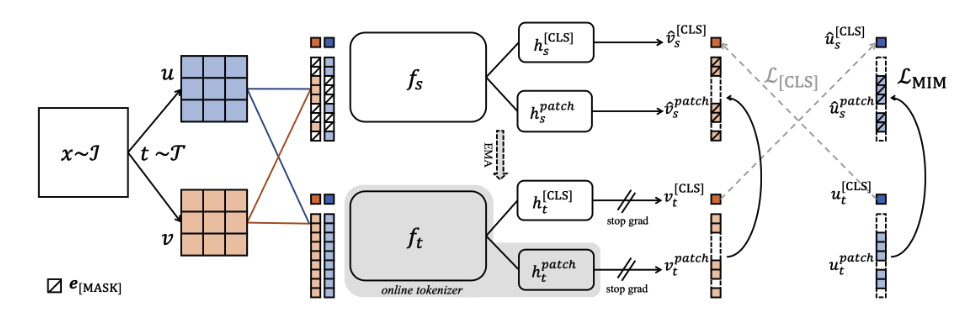
- Student and Teacher Networks: The model consists of a student network (
fs) that learns via gradient descent and a teacher network (ft) whose weights are an exponential moving average (EMA) of the student’s weights. The teacher provides stable, slowly evolving prediction targets.- the name online tokenizer stands for teacher network
- Augmented Views: For each input image, two differently augmented views,
uandv, are created. The student processes a view with randomly masked patches, while the teacher processes an unmasked view. - Stop-Gradient: Crucially, no gradients flow back through the teacher network (
stop grad). This ensures the student learns to predict the teacher’s output, not the other way around.
TRAINING Training is driven by a dual-objective loss function:
- Global Self-Distillation Loss (
L[CLS]): The global representation from the student’s[CLS]token is trained to match the global representation from the teacher’s[CLS]token. This encourages the model to learn view-invariant, high-level semantic features. - Masked Image Modeling Loss (
LMIM): The student’s patch tokens corresponding to the masked input regions are trained to predict the feature representations from the teacher’s corresponding patch tokens. This forces the model to learn fine-grained, local information.
The output are not actually patches as show in the picture. Instead, we assume that there are N classes or prototype vectors (we can assume we are predicting these prototype vector, e.g. a VQ-VAE quantization) and we get from the heads \(h_s\) a probability distribution. Then we can the cross-entropy:

CORE CONCEPT:
- DUAL CE LOSS → cross entropy loss for both CLS and Masked-patch penalization
- Masked invariance for STUDENT TEACHER rather than AUGMENTATION
3.2 Feature-Space Prediction (iBOT) vs. Pixel-Space Reconstruction (MAE)
Instead of reconstructing pixels like MAE, iBOT predicts the teacher’s feature representations. This design choice carries a distinct set of trade-offs.
| Advantages of Feature-Space Prediction (iBOT) vs input space prediciton (MAE) | Disadvantages of Feature-Space Prediction (iBOT) vs input space prediciton (MAE) |
|---|---|
| Semantic-Level Learning: Encourages capturing abstract concepts rather than low-level textures (as you do cross entropy on features not on low level pixel). | Dependency on Teacher Quality: Representations are capped by the teacher’s feature quality. |
| Robustness to Noise: Less sensitive to pixel-level noise and minor variations. | Increased Complexity: Requires maintaining and updating a teacher network via EMA. |
| Computational Efficiency: Avoids a large decoder mapping back to high-dimensional pixel space to reconstruct image. | Reduced Interpretability: Feature predictions are not directly visualizable like pixel outputs. |
| Avoids Trivial Solutions: Prevents simple blurring or interpolation strategies from satisfying the loss (you can do with pixel). | Potential Information Loss: Operating in a compressed feature space may discard fine-grained details. |
3.3 iBOT’s Evolution from BERT and BYOL
iBOT cleverly adapts and combines concepts from both its language and vision predecessors.
FROM BERT TO IBOT Compared to BERT, iBOT makes several adaptations for vision:
- self-distillation → It replaces BERT’s single-model design with a student-teacher framework. This is necessary because images lack a predefined discrete vocabulary (like words), so targets must be generated dynamically.
- dual-objective → combines masked patch prediction with global [CLS] token alignment through contrastive learning, whereas BERT relies solely on masked language modeling.
- no vocabulary →
- BERT predict token from a vocabulary → iBOT predict teacher’s continuous feature representations
- BERT tokenize via a vocabbulary → iBOT simply patchify the image without predefined discrete vocabulary
- view augmentation → IBOT relies on augmaentation views as common in visual self supervised learning (BERT does not use any augmentation)
FROM BYOL TO IBOT: Compared to BYOL, another student-teacher model,
- Approach
- BYOL focuses exclusively on matching global representations between two views
- iBOT introduces also masked token prediction.
- BYOL focuses exclusively on matching global representations between two views
- dual-level learning Impact → operating on both patch and
[CLS]tokens- forces the model to learn explicit local correspondences and spatial reasoning, a learning signal absent in BYOL (learn only global representation/feature).
- allows iBOT to build a richer, more hierarchical understanding
- source of asymmetry
- in BYOL, it comes from an added predictor head
- in iBOT it stems from the masked input to the student and the dual-objective loss
3.4 The Strategic Importance of Dual Token Representations
Maintaining separate representations for patch-level tokens and a global [CLS] token provides significant practical advantages:
- Task Flexibility: The
[CLS]token provides a ready-made global feature vector ideal for image classification, while the patch tokens can be directly used for dense prediction tasks like semantic segmentation or object detection.
4.0 Preventing Mode Collapse with Centering (TODO)
CHALLENGE A critical failure mode in self-distillation models is mode collapse, where the network learns a trivial solution by mapping all inputs to the same constant output.
- CAUSE This occurs because of a reinforcing feedback loop: if the teacher develops a slight bias towards one output dimension, the student learns to match it to minimize the loss. The teacher, being an EMA of the student, then inherits and strengthens this bias, leading to a complete collapse.
SOLUTION iBOT prevents this with a centering operation applied to the teacher’s outputs before the softmax function.
zt = softmax((ht(ft(x)) − c) / τ)
The center c is a running vector updated via an exponential moving average of the teacher’s outputs from each batch:
c ← λ · c + (1 − λ) · Ebatch[ht(ft(x))]
This simple operation has a profound effect. At equilibrium, when the training process reaches a stationary distribution, the center vector c* can be shown to converge to the mean of the teacher’s outputs over the entire dataset.
Proof of Equilibrium: At equilibrium, c* does not change:
c* = λ · c* + (1 − λ) · E[ht(ft(x))] c* - λ · c* = (1 - λ) · E[ht(ft(x))] (1 - λ)c* = (1 - λ) · E[ht(ft(x))] c* = E[ht(ft(x))]
Therefore, the centered outputs, ht(ft(x)) - c*, are guaranteed to have a zero mean over the dataset. This prevents any single output dimension from consistently dominating across all samples, effectively breaking the feedback loop and preventing mode collapse.
We now briefly turn to DINO, the final model in our overview, which provides important context for iBOT’s self-distillation mechanism.
ADD THAT IN SOME CASE YOU FIX VIA TEMEPERATURE SEE SLIDES
B. DINO and DINOv2: Knowledge Distillation with No Labels
DINO, which stands for knowledge DIstillation with NO labels, is another landmark method in self-supervised learning and a direct conceptual predecessor to iBOT’s distillation component.
- Like iBOT, it leverages a student-teacher framework with teacher as EMA of the student
- The core idea is to learn representations that are invariant to data augmentations
1. From BYOL to DINO
NB this is not contrastive as it does not explicitly defines positive pairs and negative pairs
BOOTSTRAPPING is the idea of using a model own prediction as targets to allow to learn a better model.
BYOL IDEA learns representations by training a network to predict a stable, time-delayed representation of another augmented view of the same image, so that minimizing the loss forces invariance to data augmentations rather than reliance on labels or negatives.
student:   encoder → projector → predictor → prediction
target:    encoder → projector → representation
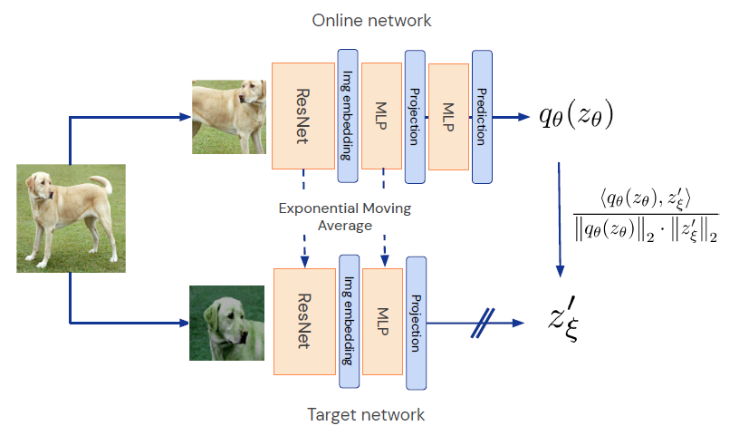
BYOL LOSS as seen above is simply the the cosine between normal image from student predictor and augmented image from EMA
CHALLENGE is mode collapse. If two network are identical they maximize the cosine similarity so they are optimal. They can be identical simply outputting a constant vector. This is called mode collapse.
BYOL doesn’t prevent collapse by saying “don’t collapse” — it prevents collapse by making collapse an unstable solution to a prediction problem.
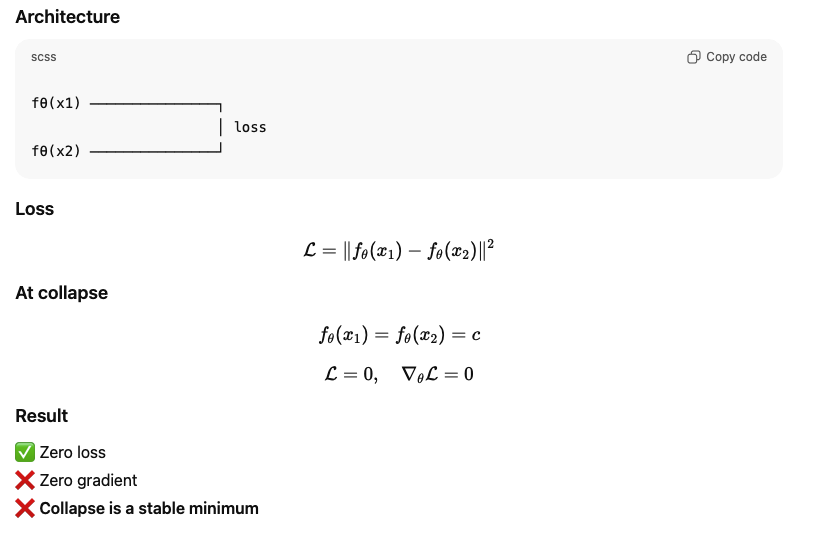
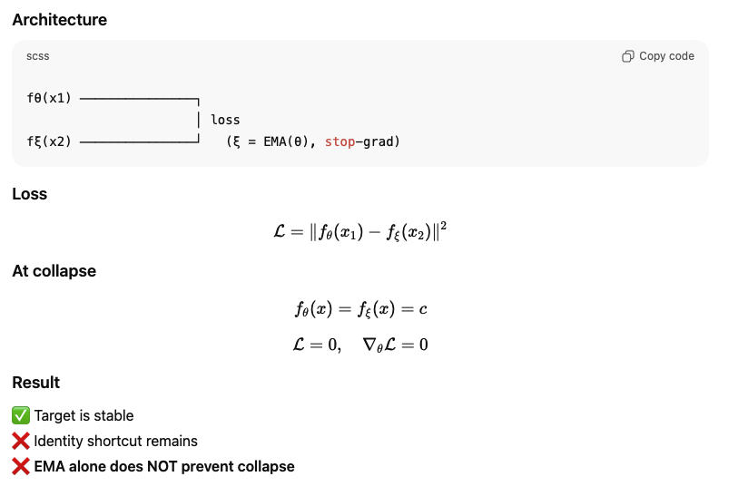
SOLUTION the solution relies on two key ingredients: EMA and PREDICTION HEAD make more constant output a non-stable solution
-
without prediction head constant output are stable optima
-
with ema is not enough
-
but with ema + prediction constant is not anymore a stable solution
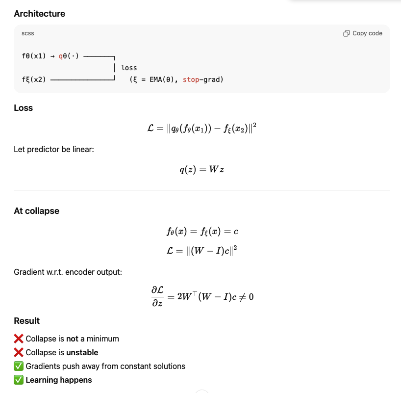
TYPE OF COLLAPSE IN DINOV1 As DINOV1 trains via a cross-entropy loss on a probability distribution divergence between teacher and student, distribution obtained from projecting CLS on a list of prototsypes (linear + softmax), there are two types of possible collapse. We define collapse learning a probability distribution that achieve a small loss but it is unrelated to the actual input:
- uniform collapse → happens when the student and the teacher start getting both a uniform distribution. This is a rolling stones, that make at each steps each other more uniform
- solution → temperature of softmax, allows you to get more sharp distribution.
- if now we have a uniform distribution, we just make a big difference from small numerical difference, which means that the distribution is highly unstable. Therefore, we are forced to commit instead of staying uniform
- solution → temperature of softmax, allows you to get more sharp distribution.
- mode collapse → we put all mass only on one item. Also this is a rolling stone.
- solution → teacher logit mean centering Just change the teacher output by keeping an ema of the mean of the logits. In this way, if the logit start to grow steadily, going towards mode collapse, also centering grows and situtation is solved
- \[f_t(x)= f_t(x) - c\]
2. From BYOL to DINO (from M.Viola + N8)
SIMILARITIES Like BYOL Dino has student–teacher framework consisting of two networks: a student that is actively trained and a teacher that is not directly optimised but updated through an exponential moving average of the student’s parameters.
- DATA AUGMENTATION DINO follows the same set of data augmentations of BYOL, i.e., a mix of horizontal flips, color jittering, grayscale conversion, Gaussian blur, and solarization.
DIFFERENCES DINO still innovate the architecture quite a bit:
- SIMPLIFIED ARCHITECTURE it removes the need for an extra prediction head, resulting in the same design for student and teacher networks:
student: encoder → projector → representation predictor → prediction target: encoder → projector → representation- Now the architecture is image encoder (VIT) + MLP (projector)
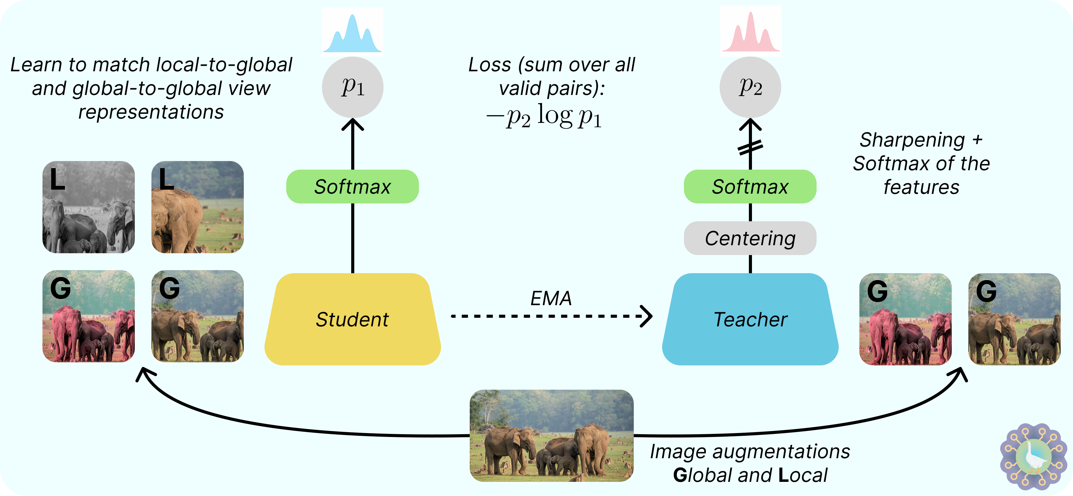
- DIFFERENT LOSS DINO uses cross-entropy to align the student and teacher output distribution instead of mean squared error or cosine similarity
- DIFFERENT INPUT HANDLING DINO follows a new multi-crop strategy: first, it generates two large crops (global, covering >50% of the image) and several smaller ones (local, <50%) from the same image.
- All crops are passed through the student network, but only the two global crops are processed by the teacher, encouraging what the authors call “local-to-global” correspondence.
- Output matching with cross-entropy happens between all valid pairs of crops, excluding identical view pairs
- NB [CLS] tokens are used for comparison of a given image crop with another
If it removes prediction, how does it avoid mode collapse?
AVOIDING MODE COLLAPSE → The always-present danger of representation collapse is prevented using two tricks: centering the teacher output by subtracting the mean computed over the batch and sharpening by dividing the sotfmax logits by a temperature T < 1.
3. From DINO to iBOT
While we introduce iBOT before DINO, it is its follow up. DINO adapted this philosophy for Vision Transformers by replacing the predictor with centering and sharpening operations on the teacher’s outputs, which proved particularly effective at producing semantic visual features and attention maps. iBOT then extended DINO’s image-level self-distillation by adding a masked image modeling objective at the patch level, combining global semantic learning with fine-grained local feature prediction in a unified framework.
- so it changed the method of DINO of producing local-to-global matching to masked matching
- DINO’s centering/sharpening mechanism (instead of a predictor) produces richer semantic structure especially in ViTs
- e.g., yielding attention maps that naturally segment objects without any supervision—making features more interpretable and semantically meaningful.
4. DINOV2
4.1 From iBOL to DINOV2
DINOv2 scales up iBOT’s to create a robust, general-purpose foundation model approach with:
- a carefully curated 142M image dataset
- longer training
- architectural refinements
4.2 DINOV2 Innovations
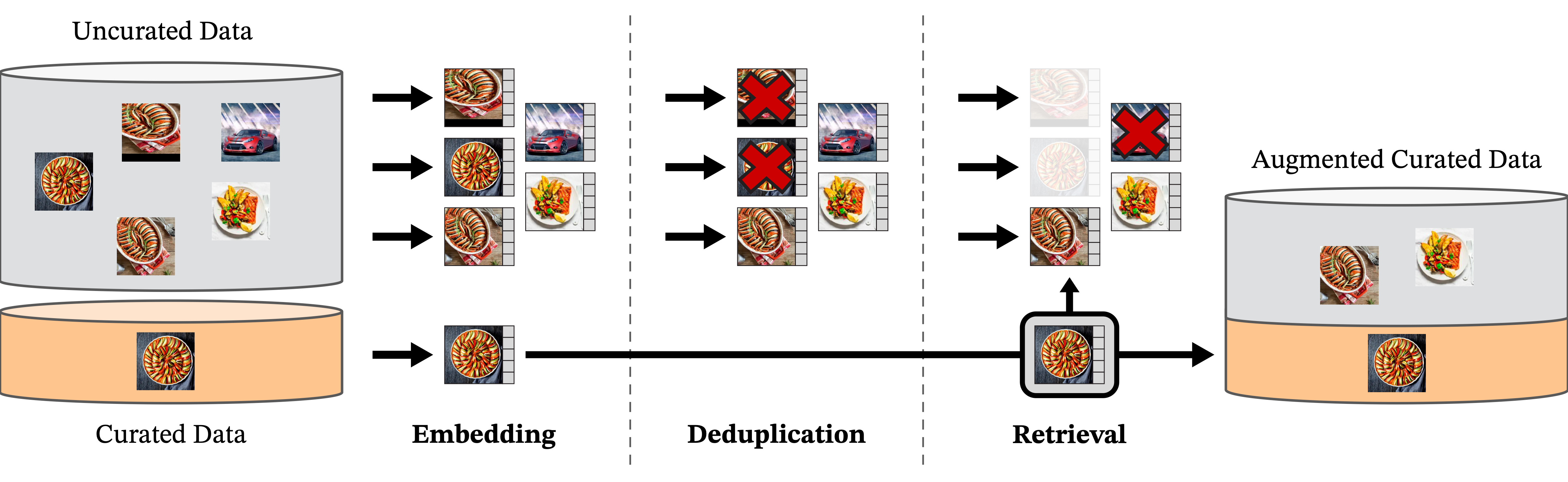
DATASET DINOv2 made the choice to prioritize quality over quantity: it builds its own curated dataset, named LVD-142M, starting from an initial set of ~1.2B web images. The pipeline:
- build high quality dataset using curated sources (e.g., imagenet 1k)
- filter near-duplicate images with a copy detection pipeline
- retrieve similar image (so high quality) from bigger dataset with selecting the k-nearest neigh (k=4)
TRAINING is a combination of loss and desiderata:
- global and view-invariant reprsentation → use cross-entropy comparison as in DINO, where student and teacher compare [CLS] token features from different crops of the same image.
- local-information → use the iBOT prediction of masked patches
- increase pixel level precision → use mixed resolution (namely pass e.g. to some 518x518 high resolution compared to 256x256 standard). This boost the final granularity of the local features and increase performance on dense task such as segmentation
ARCHITECTURE Also here there are some difference
- mixed MLP → A trick used is to use different head from the output of the encoder. Also DINO used a projection head, but now we have different head for CLS and local patches, to avoid interference
- Improved centering and feature regularization → the original teacher centering + sharpening is replaced by a special batch normalization (
Sinkhorn-Knopp centering). Furthermore, a regularizer that encourages features to be uniformly spread out on the unit sphere is added (KoLeo). This acts on the [CLS] projections of the first global crops within the batch, representative enough to enforce feature spread.
LOSS This is the final loss that is been optimized

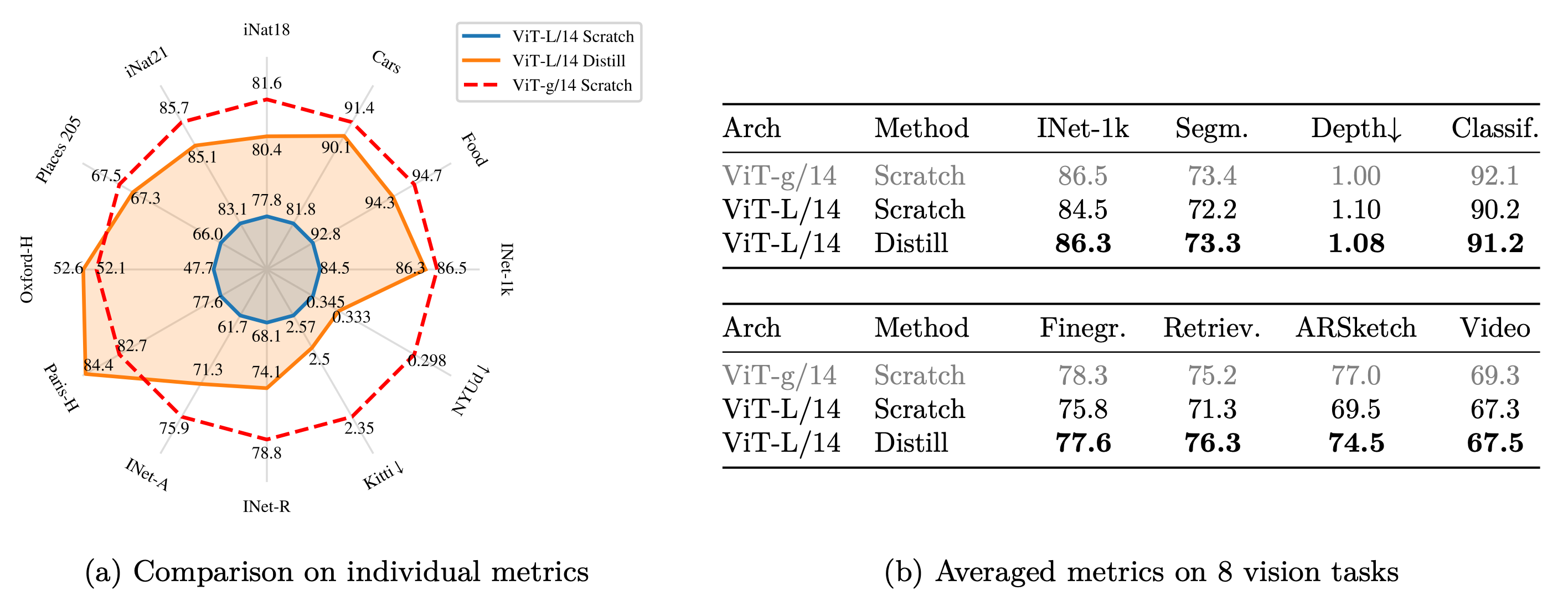
KNOWLEDGE DISTILLATION Rather than training different version from scratch, train firstly the biggest and use it as teacher:
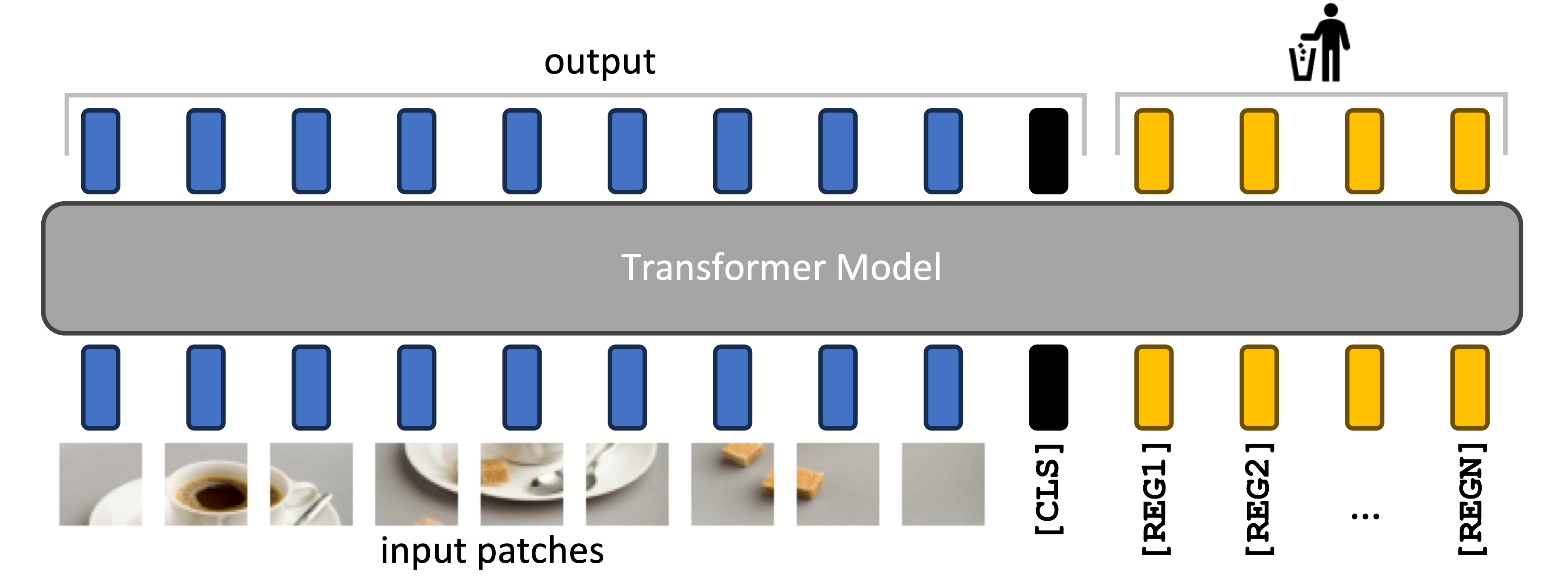
VISION REGISTERY this are some tokens add to the input to capture global info on top of the CLS
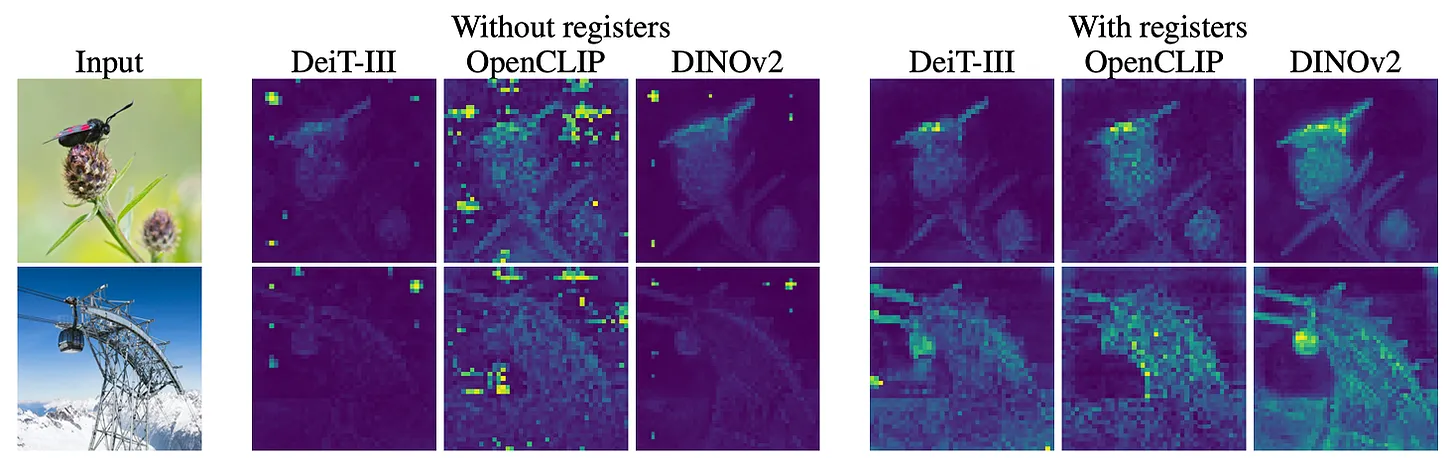
Indeed, once we train too much we still improve accuracy on sparse info task as classification on imagenet. But our performance decreases dramatically on dense task such as segmentation. This is because some patches hidden representation becomes very high-norm as full of information. This normally are useless background patches that transformer smartly use as blank spaces where to write global informations to carry complex reasoning
4.3 DINOV2 Experiments
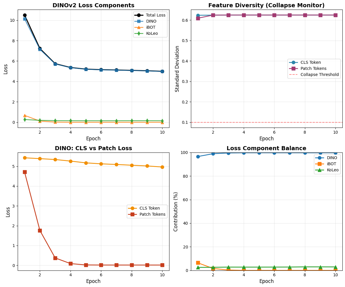
LOSSES COMPARISON:
- DINO loss (therefore CE between EMA and teacher for crops) dominates showing self-distillation is the primary learning mechanism
- iBOT’s rapid decay suggests masked modeling only helps bootstrap initial features
- KoLeo’s negligible impact means the architecture inherently resists collapse.
MODE COLLAPSE both CLS and patch tokens maintain high diversity (0.64) far above collapse threshold. Identical diversity levels indicate well-balanced global/local representations with no feature degeneration.
PATCH VS CLS patch features converge way faster than CLS tokens. Local patterns are easier to learn; global semantic understanding requires sustained refinement
4.4 DINOV2 Core Code
Teacher Init
self.student = TinyViT(**model_config).to(device)
self.teacher = TinyViT(**model_config).to(device)

# 1. Load the same init of studen
self.teacher.load_state_dict(self.student.state_dict())

# 2. Teacher doesn't need gradients
for p in self.teacher.parameters():
    p.requires_grad = False

# 3. Teacher is in eval mode
self.teacher.eval()
Teacher Update
@torch.no_grad()
def update_teacher(self):
	"""EMA update of teacher weights"""
	for param_s, param_t in zip(self.student.parameters(), self.teacher.parameters()):
	    param_t.data.mul_(self.momentum).add_(param_s.data, alpha=1 - self.momentum)
Centering is done only for the CLS output of the teacher
def update_center(self, teacher_cls):
  """Update center for teacher CLS outputs only (DINOv2 change)"""
  # EMA update
  cls_center = teacher_cls.mean(dim=0, keepdim=True)
  self.center_cls = self.center_cls * self.center_momentum + cls_center * (1 - self.center_momentum)
iBOT masking → an important details is that masking is applied only in the student forward pass and only on one of the two global crop (and none for the locals)
def generate_mask(self, batch_size):
	"""Generate random mask for iBOT (masked image modeling)"""

	num_masked = int(self.ibot_mask_ratio * self.num_patches)
	mask = torch.zeros(batch_size, self.num_patches, dtype=torch.bool, device=device)

	for i in range(batch_size):
	    # Random masking for each sample
	    masked_indices = torch.randperm(self.num_patches)[:num_masked]
	    mask[i, masked_indices] = True

	return mask
DINO Losses
def dino_loss(self, student_output, teacher_output):
  """
  Stable cross-entropy for DINO:
  - student_output: B x D
  - teacher_output: B x D
  ----
  return scores B
  """
  # get prob distribution and log prob
  student_out = F.log_softmax(student_output, dim=-1)
  teacher_out = F.softmax(teacher_output, dim=-1)
  # compute ce for each batch and take mean accross batches
  return -(teacher_out * student_out).sum(dim=-1).mean()

# inside forward -> skip first global where you apply iBOT loss
if not_first_global:
	loss += dino_loss(self, student_cls, teacher_cls)
	# treat patches as batch
	loss += dino_loss(self, student_local.reshape(-1, hidden_dim),teacher_local.reshape(-1, hidden_dim))
iBOT Loss is literally dino → NB how this is applied to each patch and the patched image is treated as a batch dimension
 if self.ibot_weight > 0 and ibot_mask is not None:
    # Extract masked patch predictions from first global crop
    # Student: predictions at masked positions
    student_masked = student_patch[0][ibot_mask]  # [num_masked_total, out_dim]

    # Teacher: ground truth at masked positions
    teacher_masked = teacher_patch[0][ibot_mask]  # [num_masked_total, out_dim]

    # Temperature scaling for iBOT
    student_masked = student_masked / self.student_temp
    teacher_masked = teacher_masked / current_temp

    # Compute loss only on masked positions
    loss_ibot = self.dino_loss(student_masked, teacher_masked)