Notes on World Models
A. World Models (L12)
In this paragraph we are going to introduce world models.
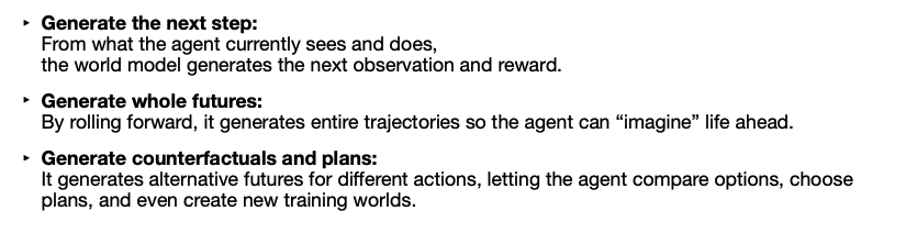
- World models are generative model that learn a probability distribution over a state space.
- World models are therefore encouraged to learn rich internal representations of environment.
- These internal representations allows for predicting future state in down-stream task such as planning and decision-making
NB, in world models generation means simulating how the world evolves over time:
Mental Models
World models : Mental model = AI Agent : Human Agent While mental model comes from cognitive psychology / philosophy and they are necessarily the same thing as world model, they play for human a similar role than the one played by world models for AI Agent. Indeed, mental model are a simplified model of reality which allow us to quickly:
- predict future before based on possible actions (”if i do X, then Y will happen”)
- integrate different elements such as perception, memory, and knowledge
- adaptive they are easily update based on new evidence
A human world model is not a static library of facts but a flexible and ever-evolving mental construct rooted in perception and memory
Furthermore, our mental models require a ton of data. A four year-old child has seen more data than an LLM!
The First World Model (Dyna)
1. Reinforcement Learning Context
There are two main type of RL Algorithms:
- model-free RL which are for example (Q-Learning, SARSA, Reinforce). They do not learn a transition matrix, therefore they do not learn \(P(S \vert a,s)\). Instead they learn a quality function that tells you how good is either a state (\(V(s)\)) or a state-action pair (\(Q(s,a)\)).For example the idea of Q-Learning is to act with the world and learn time by time this quality function. While we learn we sample whether to act at random or according to them
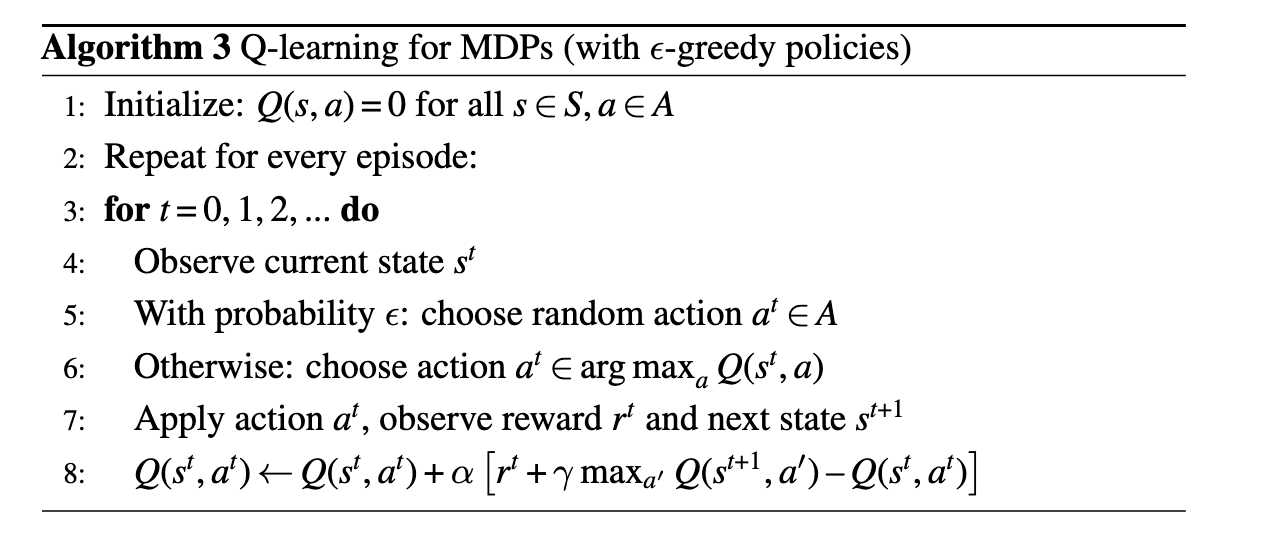
I don’t know the rules of the game. I just remember which moves worked. So i need to try and learn
- model-based RL, for example → DP, Value Iteration, Policy Iteration. You learn a model of the environment \(P(S \vert a,s)\). In Value Iteration for example you use that probability model \(P(S \vert s,a)\) to pick the action that maximize the expected reward based on an optimal value function \(V^*\):

I learned the rule of the game before, so I can think instead of trying. I can play instead of learn
2. Sutton Invented Dyna
On the contrary to the two paradigm DYNA is both model-based and model-free. Like model-based architecture it has a model of the environment \(M(s,a) \sim P(S \vert s,a)\) which allows to predict next state. But differently from model-based RL it is not learned before and used to sample actions. Instead, it is used to generate fake trajectory, which are used to update Q(s,a) as in Q-Learning. Actions are chosen as in Q-Learning either at random or argmax_a Q(s,a)
Dyna is a hybrid RL architecture that learns a model of the environment like model-based RL, but uses it to generate simulated experience for model-free updates.
Initialize Q(s,a)
Initialize Model(s,a)

repeat for each real step:
    observe s
    choose a using ε-greedy(Q)
    execute a in real world
    observe r, s'

    // 1. Real experience update
    Q(s,a) ← Q(s,a) + α [ r + γ max_a' Q(s',a') − Q(s,a) ]

    // 2. Learn the model
    Model(s,a) ← (r, s')

    // 3. Planning with fake experience
    repeat N times:
        sample (ŝ, â) from previously seen state–action pairs
        (r̂, ŝ') ← Model(ŝ, â)
        Q(ŝ,â) ← Q(ŝ,â) + α [ r̂ + γ max_a' Q(ŝ',a') − Q(ŝ,â) ]

    s ← s'
The learned M(s,a) is a world model for the agent.
Schmidhuber Invented World Models
Core Idea
Schmidhuber propose to organize AI Agents into three fundamental modules:
- Vision (V) elaborate perception. E.g., if vision, maps input images from agent’s sensors to compressed low dimensional latent vectors
- Memory (M) it take as input previous memory and current compressed (by V) sensorial information and update the current memory
- Controller (C) it decide which action to take based on current compressed sense (V) and memory info (M)
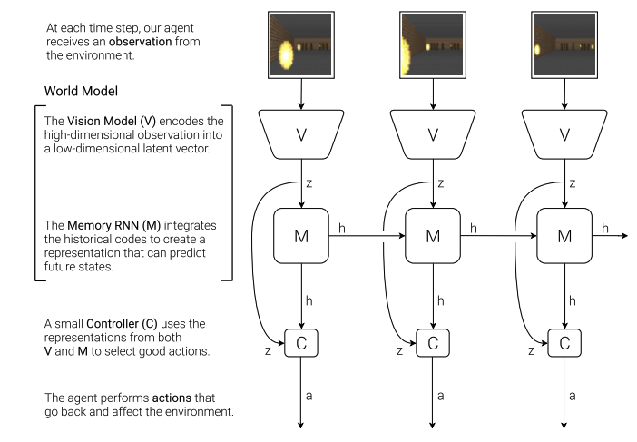
Let′s outline some terminology for this chapter:
- x → observation, 64 x 64 x 3 image
- z → latent code from the V
- q(z|x) → encoder distribution from V
- p(z) → prior on latent distribution from V (standard normal)
- p(x|z) → decoder distribution from V
- h → memory outputted by sampling the M
- a → action
- r → reward
Advantage of Equipping Agent with World Model
Explicit World Modelling can help convergence of policy as we need to update only the tiny model with the reward signal, which uses already informative representations (V+M) learned via self-supervision.
As written above the core benefit is that we use a very tiny controller, rather than a massive one (as normal in DeepRL). So only this tiny guy is trained with signal from RL. This signal is noisy so it was problematic to tune milions of params as in DRL. Instead, we tune the massive guys (V,M) via self-supervised learning
Usage of World Model
To train V and M, we collect some history of type \((a_i,x_i)_0^{t=10k}\) by random actions. Now for training:
- V → we just need \(X\)
- M → we create a new dataset by passing X → V(X) = Z. Then we feed to M the current compressed vision \(z_i\), the memory up to know \(h_{i}\), and the action taken \(a_{i}\) and we teach it to predict what is going to be the future compressed sensed V′s output (so M input), that is \(z_{i+1}\)
- C → we have two usage that share the usage of CMAES for training given the reward signal:
- complete dreaming (DOOM Game): we use the collected training history playing at random to train both V,M. After we train the controller by using the future predicted by M as future input of M, creating a circle in the world model of imagined states. Nevertheless, M requires both \(z\) and \(a\) as actions → indeed, we use the a found by the policy (finally, the reward \(r(z)\) is implemented by defualt in openai ennvironment).
- augmented perception (Cars Game): compared what happen if we trained C in a real world when the input is only z from V, or when we augment it via M. It seems, world model aka memory augmentation helps a lot in the task
See here the rollout and training dynamics:
The code
# --- Setup ---
z_dim = 32
action_dim = 3
hidden_dim = 256

vae = V(z_dim=z_dim)
rnn = M(z_dim=z_dim, action_dim=action_dim, hidden_size=hidden_dim)
controller = Controller(z_dim=z_dim, hidden_size=hidden_dim, action_dim=action_dim)

# --- Stage 1: Train VAE ---
# Gather 10,000 random rollouts, train VAE to reconstruct frames
# optimizer_vae = torch.optim.Adam(vae.parameters())
# for batch in data:
#    recon, mu, logvar = vae(batch)
#    loss = vae_loss(recon, batch, mu, logvar)
#    loss.backward()

# --- Stage 2: Train Memory (RNN) ---
# Use trained VAE to encode all frames into Z. Save (z_t, a_t, z_{t+1}) tuples.
# optimizer_rnn = torch.optim.Adam(rnn.parameters())
# for z_t, a_t, z_next in latent_data:
#    pi, mu, sigma, _ = rnn(z_t, a_t)
#    loss = mdn_loss(pi, mu, sigma, z_next)
#    loss.backward()

# --- Stage 3: Train Controller (Evolution) ---
# VAE and RNN are now FROZEN. We only train the Controller's weights.
# Since we can't backprop reward easily through the environment, we use
# Evolution Strategies (CMA-ES) instead of Gradient Descent.

def run_rollout(controller, env):
    obs = env.reset()
    h = torch.zeros(1, 1, hidden_dim) # RNN hidden state
    c = torch.zeros(1, 1, hidden_dim) # RNN cell state

    done = False
    total_reward = 0

    while not done:
        # 1. Vision: Encode frame
        obs_tensor = torch.tensor(obs).permute(2,0,1).unsqueeze(0).float() / 255.0
        with torch.no_grad():
            mu, logvar = vae.encode(obs_tensor)
            z = vae.reparameterize(mu, logvar)

        # 2. Control: Decide action based on Vision (z) + Memory (h)
        with torch.no_grad():
            action = controller(z, h[0]) # Pass hidden state h (not c)
            action = action.squeeze().numpy()

        # 3. Environment Step
        obs, reward, done, _ = env.step(action)
        total_reward += reward

        # 4. Memory: Update hidden state for next step
        # RNN predicts next Z (we ignore the prediction, we just want the new h)
        action_tensor = torch.tensor(action).view(1, 1, -1)
        z_tensor = z.view(1, 1, -1)
        with torch.no_grad():
            _, _, _, (h, c) = rnn(z_tensor, action_tensor, (h, c))

    return total_reward

# Evolution loop would repeatedly call run_rollout with different controller weights
Vision Module
The V module is a straightforward VAE model.
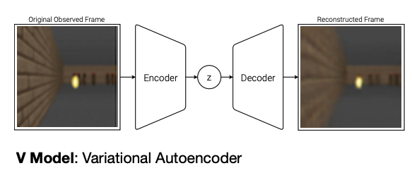
It learn to minimize a reconstruction term (e.g., the likelihood that the decoder generate the input data) and it uses a regularizer to force normality (required to sample from z afterwards, and to force the encoder q to actually learn a distribution rather than memorizing)
\[L_{VAE} = \mathbb{E}_{q(z|x)}[\log p(x|z)] - D_{KL}(q(z|x)||p(z))\]NB, if you model the pixel generation of the decoder p(x| μ, σ) as a normal maximizing the log-likelihood is equivalent to minimize the MSE
The code
class V(nn.Module):
    def __init__(self, img_channels=3, z_dim=32):
        super(VAE, self).__init__()

        # Encoder
        self.enc_conv = nn.Sequential(
            nn.Conv2d(img_channels, 32, 4, stride=2), nn.ReLU(),
            nn.Conv2d(32, 64, 4, stride=2), nn.ReLU(),
            nn.Conv2d(64, 128, 4, stride=2), nn.ReLU(),
            nn.Conv2d(128, 256, 4, stride=2), nn.ReLU()
        )
        self.fc_mu = nn.Linear(2*2*256, z_dim) # get mean
        self.fc_logvar = nn.Linear(2*2*256, z_dim) # get variance

        # Decoder
        self.dec_fc = nn.Linear(z_dim, 2*2*256)
        self.dec_conv = nn.Sequential(
            nn.ConvTranspose2d(256, 128, 5, stride=2), nn.ReLU(),
            nn.ConvTranspose2d(128, 64, 5, stride=2), nn.ReLU(),
            nn.ConvTranspose2d(64, 32, 6, stride=2), nn.ReLU(),
            nn.ConvTranspose2d(32, img_channels, 6, stride=2), nn.Sigmoid()
        )

    def encode(self, x):
        h = self.enc_conv(x)
        h = h.view(h.size(0), -1)
        return self.fc_mu(h), self.fc_logvar(h)

    def reparameterize(self, mu, logvar):
        std = torch.exp(0.5 * logvar)
        eps = torch.randn_like(std)
        return mu + eps * std # sample the encoder

    def decode(self, z):
        h = self.dec_fc(z)
        h = h.view(h.size(0), 256, 2, 2)
        return self.dec_conv(h)

    def forward(self, x):
        mu, logvar = self.encode(x)
        z = self.reparameterize(mu, logvar)
        recon_x = self.decode(z)
        return recon_x, mu, logvar # return a distribution over the x

# Loss: Reconstruction + KL Divergence
def vae_loss(recon_x, x, mu, logvar):
    BCE = F.mse_loss(recon_x, x, reduction='sum') # prefered to log-likelihoof
    KLD = -0.5 * torch.sum(1 + logvar - mu.pow(2) - logvar.exp())
    return BCE + KLD
Memory Module
The memory module is trained via attaching a MDN (mixed density network with 5 gaussians) instead of final linear layer to the output of the RNN
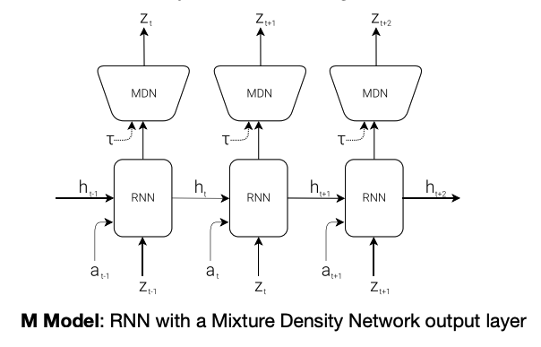
This trick allows us to treat the RNN output as parametrization for a gaussian, and rather than having 1 predicted \(\hat z_{i+1}\) we will have a distribution where to sample many, which is what we want from our generative world models. Therefore we train by minimizing the following function
\[L = - \log \left( \sum_{k=1}^5 \pi_k \mathcal{N}(z_{t+1} | \mu_k, \sigma_k) \right)\]with π,μ,σ be a projection of RNN(zᵢ) output.
The code
class M(nn.Module):

    def __init__(self, z_dim=32, action_dim=3, hidden_size=256, n_gaussians=5):
        super(MDNRNN, self).__init__()
        # hyperpam
        self.z_dim = z_dim
        self.n_gaussians = n_gaussians

        # core network
        self.lstm = nn.LSTM(z_dim + action_dim, hidden_size, batch_first=True)

        # Mixture Density Network Heads -> simply output how may, their mean, and std
        # not standard -> each feature of output vector is modelled
        # by 5 gaussian
        self.fc_pi = nn.Linear(hidden_size, n_gaussians * z_dim) # probability that is modelled by gaussian 1,2,3,4,5
        self.fc_mu = nn.Linear(hidden_size, n_gaussians * z_dim)
        self.fc_sigma = nn.Linear(hidden_size, n_gaussians * z_dim)

    def forward(self, z, action, hidden=None):
        # Input: Concat current latent z and action a
        x = torch.cat([z, action], dim=-1) # [Batch, Seq, Z+Action]
        output, hidden = self.lstm(x, hidden)

        # Output parameters for GMM
        pi = F.softmax(self.fc_pi(output).view(-1, self.n_gaussians, self.z_dim), dim=1)
        mu = self.fc_mu(output).view(-1, self.n_gaussians, self.z_dim)
        sigma = torch.exp(self.fc_sigma(output)).view(-1, self.n_gaussians, self.z_dim)

        return pi, mu, sigma, hidden

# Loss: Negative Log Likelihood of the true next_z
def mdn_loss(pi, mu, sigma, next_z):
    # next_z shape: [Batch*Seq, Z_dim] -> Expand for Gaussians
    target = next_z.unsqueeze(1).expand_as(mu)

    # Gaussian Probability Density Function
    prob = (1.0 / (sigma * (2 * torch.pi)**0.5)) * torch.exp(-0.5 * ((target - mu) / sigma)**2)

    # Weighted sum over mixture components
    prob = torch.sum(prob * pi, dim=1)

    # Negative Log Likelihood
    nll = -torch.log(prob + 1e-8)
    return torch.mean(nll)
Controller Module
The idea:
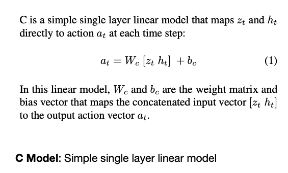
The code
class Controller(nn.Module):
    def __init__(self, z_dim=32, hidden_size=256, action_dim=3):
        super(Controller, self).__init__()
        self.fc = nn.Linear(z_dim + hidden_size, action_dim)

    def forward(self, z, h):
        # Concatenate Vision (z) and Memory (h)
        inp = torch.cat([z, h], dim=-1)
        return torch.tanh(self.fc(inp)) # Actions usually in range [-1, 1]
Type of World Models
In a world model ideally the environment is characterized by two quantities:
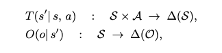
\(T\) maps state of the environment s and action of the controller to new state of the environment. Instead, \(O\) maps state of the environment to observation of the agent.
In World Model 2018 the observation are the pixel (so the input of the visionary V routine). Instead, the states are [z, h] the input of the control C, namely memory and compressed input. The memory maps action and state (z) to a new state (z’), being therefore insensible to observations.
These are the 4 main types of world models and their most popular exmaples:
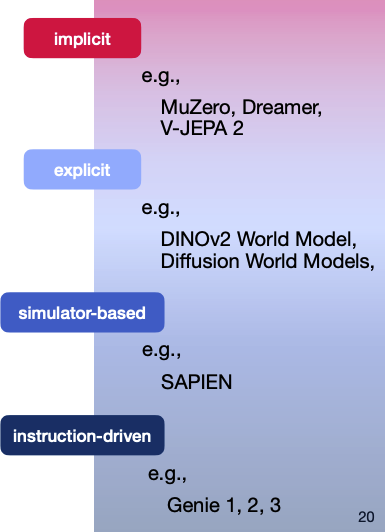
Implicit world Model
CORE IDEA Agent′s world model maps from latent observation to latent future observatios. Therefore, it never generate in the same domain of the ambient of the agent (e.g., pixel), but state of this world model are latent vectors of a deep learning aarchitecture. It is called latent dynamic function:
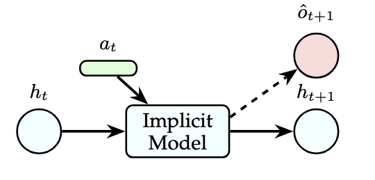
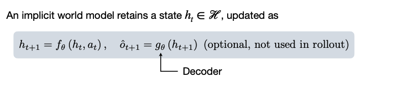
- The decoder is useful only for training, and it is never used to actually reconstruct state into the original one (if not for paper viz)
- Therefore, agent does not reconstruct latent states in observation during planning.
Thinking in abstract symbols about the game state, without ever “rendering” a picture of the board
MuZero
CORE IDEA integrates a learned latent dynamics model with Monte Carlo Tree Search. It use this latent dynamic model to imagine future trajectories, and MCTS in the sense that it picks few best actions to create few future trajectories in paralle . At each step/node it use the policy to chose an action, it uses the latent dynamic model to predict the future state, and it applies a reward function on this action and future state. It choose finally the action that has been chosen most time (rather than the one with highest short term reward)
Use learned latent dynamic for planning (pick best action) at decision time
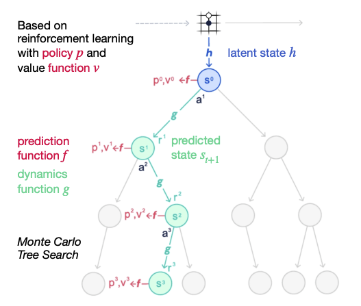
ARCHITECTURE MuZero learns three functions:
-
ha representation function that maps the initial observation to a latent state -
ga dynamics function that predicts the next latent state -
fa prediction function that outputs a policy (distribution over action) and a value estimate (expected reward of keep playing from that latent state) from a latent state.
DreamerV3
CORE IDEA The core idea of Dreamer is to learn a latent dynamics model of the environment from real experience and then use this model to generate imagined future trajectories entirely in latent space. These imagined trajectories are used to optimize a policy and a value function, allowing the agent to improve its behaviors without interacting with the real environment at every update.
Learn a latent dynamic, generate a lot of trajectory (before decision time), train your policy on these trajectories
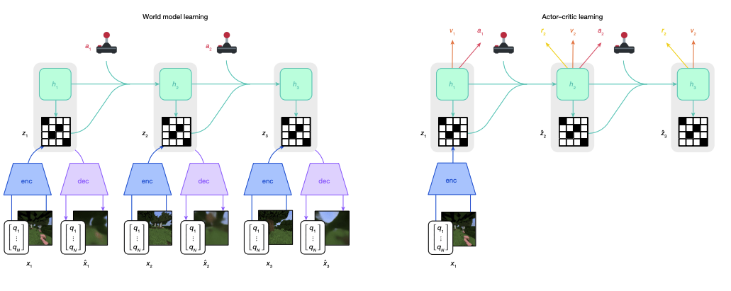
(in the image: the encoder is what we train and it has a deterministic hidden output h and a stochastic z. The stochastic is reconstructed into x by the decoder to train the encoder via MSE)
ARCHITECTURE The world model in Dreamer is implemented as a recurrent state-space model that combines deterministic and stochastic components. The deterministic hidden state captures information that is predictable from past experience, while the stochastic latent variables model uncertainty and variability in the environment.
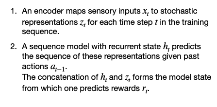
TRAINING Observations are encoded into latent variables during training, and the recurrent dynamics model predicts how these latents evolve given actions.
MUZERO VS DREAMER MuZero is especially effective in discrete action spaces with well-defined planning horizons, while Dreamer scales more naturally to continuous actions and long-horizon control tasks. Both approaches demonstrate that accurate prediction of raw observations is not necessary for strong performance, as long as the latent dynamics capture the aspects of the environment that matter for decision-making.
JEPA Models (N11)
While JEPA models are still implicit world models, we will make a deep dive in their structure.
I-JEPA Core Idea
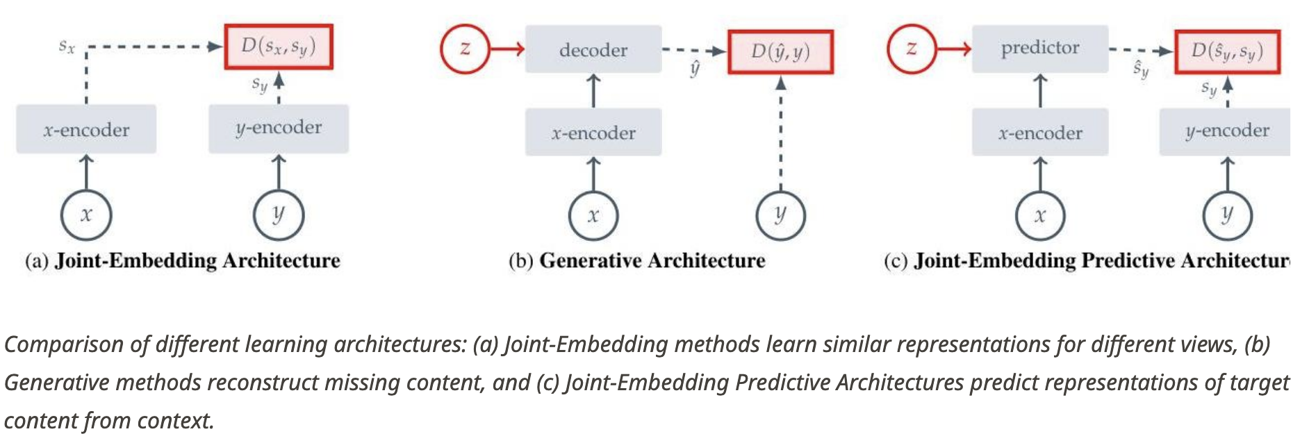
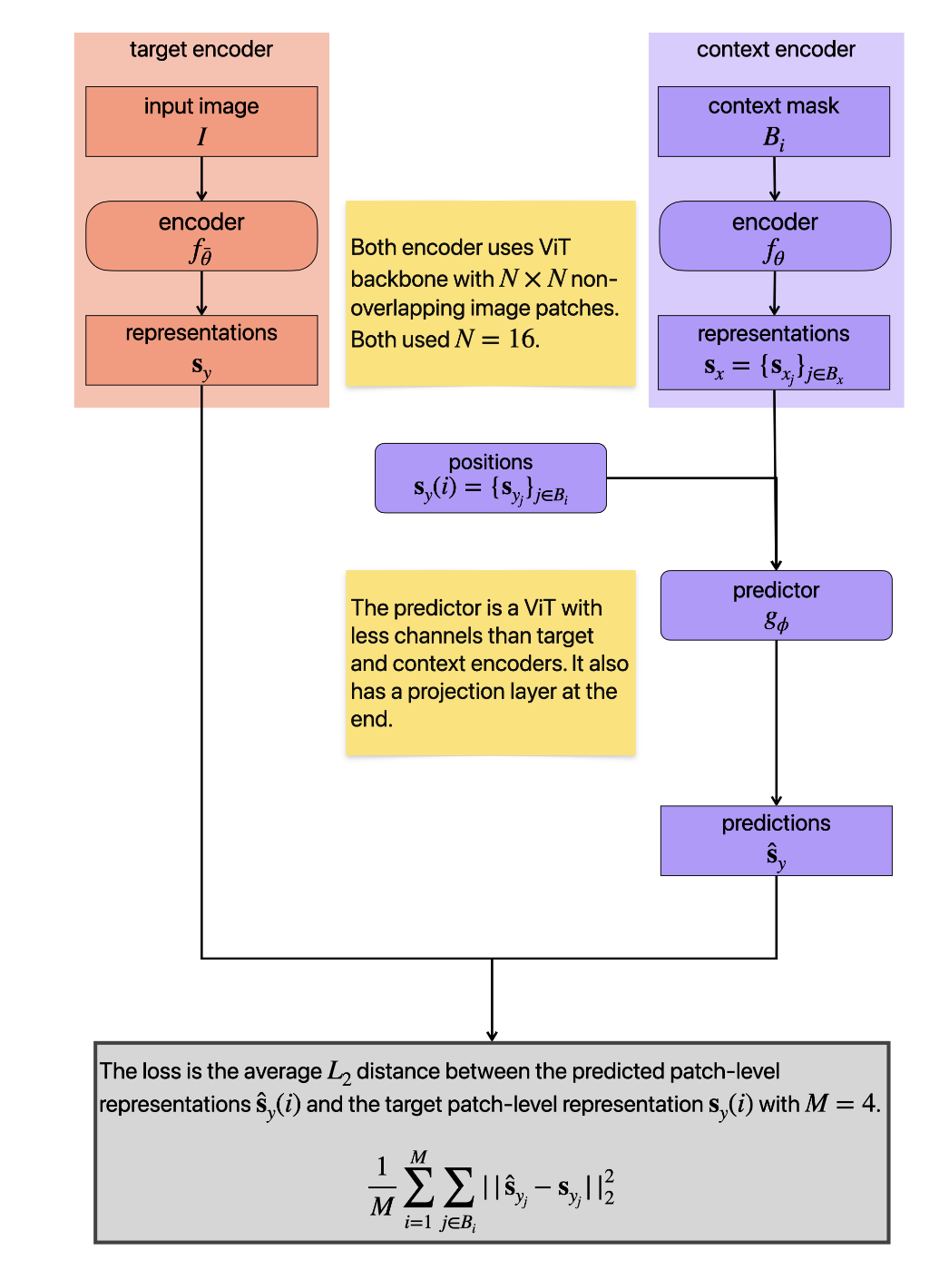
I-Jepa is a joint embedding predictive architecture. Such architecture learn meaningful representation by trying to match masked representations of a student model with masked representation of a teacher model.
INTUITION: JEPA predicts abstract representations rather than raw high-dimensional inputs, avoiding modeling irrelevant details
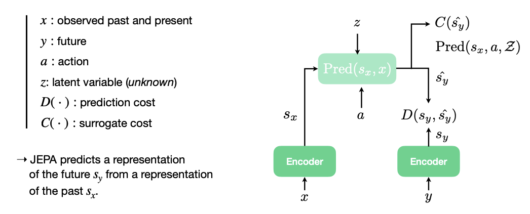
Predictor project student output in joint embedding with teacher and is used to avoid mode collapse as in BYOL, iBOT, DINO…
There are a lot of details here:
- differently from simple joint embedding architecture (see BYOL) or contrastive methods (SIMCLR), JEPA do not work with two different version of the same input where difference relies on different augmentation → no explicit look for representation invariance.
- differently from masked autoencoder, model performance are not checked by reconstructing pixel image and checking mean squared error. Rather, they MSE is measured between patch-level hidden representation of the predictor and the teacher encoder. So, everything happens in a joint embedding space.
INNOVATION: JEPA take student-teacher comparison from contrastive methods and masking from MAEs. It leaves augmentation of contrastive methods and reconstruction via decoder of MAEs
I-JEPA Tokenization
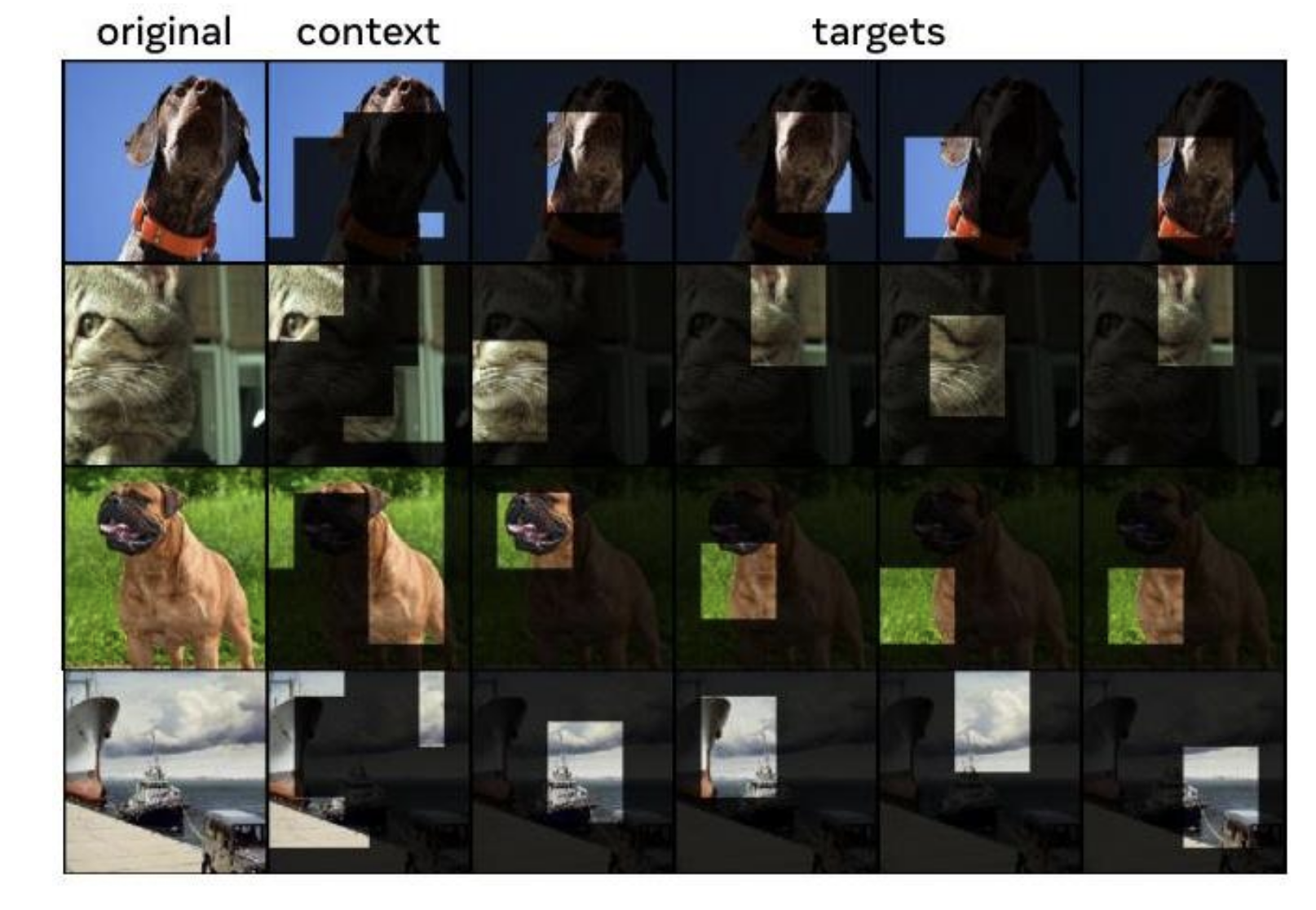
MASK The first intuition is that here masks are not the covered but the used part of the image. It is a bit counterintuitive, but these masks are indices used to select patches from the image.
MASKING ALGORITHM A tricky detail of I-JEPA lies in the way it tokenize the image. The algorithm is:
- sample for each image
Tmasks made byKtpatches→ _each mask is a big rectangles (_much bigger than what we used in MAEs) - sample for each image
Mmasks made byKcpatches:- each context mask of the M is used to predict each target mask
- we explicitely never pick patches (masks) already present in the target to avoid dumb tasks
I-JEPA Forward Pass
Once we created the masks the image masks we can use it in the forward pass.
The core intuition is to the context mask patches to predict each of the target mask patches
The forward pass follow this logic:
- select patches via context encoder masking
- pass through the encoder
- append position embeddings of the patches of the target masks to the encoder output
- this is done so that the predictors know which patch predict
- pass through the predictor to get as output as many vector as target mask patch
- now we are in the joint embedding shared between the predictor and
- compute target patches via target encoder
- compute loss
I-JEPA Training
Differently from what is shown above the loss used by I-JEPA is smooth-l1 rather than l2 loss.
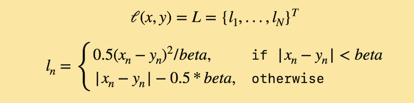
The context_decoder is clearly not trained by updated via an EMA of the context encoder:
def ema_update(context_encoder, target_encoder, beta):
    """
    for each parameter pair (context_param, target_param):
        target_param = beta * target_param + (1 - beta) * context_param
    """
    # loop through parameters
    with torch.no_grad():
        for student_param, teacher_param in zip(context_encoder.parameters(), target_encoder.parameters()):
            # we need .data otherwise "target_param = something" will not write in the model
            # we need .add_ and .mul_ to not create copy in memory
            teacher_param.data.mul_(other=beta).add_(other=student_param.data, alpha=1 - beta)
I-JEPA Code Implementation
The two core part of the code implementation is useful to understand is the masking code and the forward passes of the encoder_context/_target (same model) and the predictor. Both are ViTs.
MASKING CODE
The mask are not bool mask but list of index. Using advanced indexing of torch we can extract relevant patches:
def apply_masks(x, masks): # TODO: add study
    """
    :param x: tensor of shape [B (batch-size), N (num-patches), D (feature-dim)]
    :param masks: *list* of tensors containing indices of patches in [N] to keep
    """
    # len(m) -> number of patches sample for a mask view (context)
    # len(mask) -> number of masked views created for a single imaged
    all_x = []
    for m in masks:
        mask_keep = x[:,m,:] # B, len(m), D
        all_x.append(mask_keep)
    return torch.cat(all_x, dim=0) # [len(masks) * B, len(m), D]
To decide what we are going to select for masking we pass to parameters: (i) Area percentage and H/W ratio (describe how much of a fat or tall matrix we pick). Then selecting the mask size is possible solving the following equations (\(H\) and \(W\) are patch_h and patch_w, \(h_m\) and \(w_m\) are the mask dimensions to compute):
-
Area constraint: The mask should cover a fraction \(s\) of the total area: $$ h_m \cdot w_m = s \cdot H \cdot W
$$
-
Aspect ratio constraint: The mask should have aspect ratio \(r\): \(\frac{w_m}{h_m} = r\)
Then we get the code
def get_mask(patch_h, patch_w, scale, aspect_ratio):
    """
    :param patch_h: number of patches along height
    :param patch_w: number of patches along width
    :param scale: scale of the mask with respect to the image (0 to 1)
    :param aspect_ratio: aspect ratio of the mask (width / height)
    :return: height and width of the mask
    """
    mask_h = int(round(math.sqrt(scale * patch_h * patch_w / aspect_ratio)))
    mask_w = int(round(math.sqrt(scale * patch_h * patch_w * aspect_ratio)))

    # clamp to valid dimension -> a mask cannot be larger than the image itself, wrong inputting can cause it
    mask_h = min(mask_h, patch_h)
    mask_w = min(mask_w, patch_w)

    return mask_h, mask_w
The last element that we need is how to sample an image to get this mask. The idea is easy. An image is tokenized in this way, e.g. for an image described by 2x2 grid of patches we get patch assembled h1w1,h1w2,h2w1,h2w2 . So once we have the mask height and width (via get_mask) we sample a valid beginning on h and w . NB if we move on the patchified image made as a list of pixels we access the patch at h=j and width=i via: j*patch_h +i*patch_width
def get_context(patch_dim, aspect_ratio, scale, target_patches):
    patch_h, patch_w = patch_dim
    block_h, block_w = get_mask(patch_h, patch_w, scale, aspect_ratio)

    #get a random starting patch
    start_patch_h = torch.randint(0, patch_h - block_h+1, (1,)).item()
    start_patch_w = torch.randint(0, patch_w - block_w+1, (1,)).item()
    start_patch = start_patch_h * patch_w + start_patch_w

    #get the patches in the context_block
    patches = []
    for i in range(block_h):
        for j in range(block_w):
            if start_patch + i * patch_w + j not in target_patches: #remove the target patches to avoid overlapping
                patches.append(start_patch + i * patch_w + j)
    context_patches = [torch.tensor(patches)]
    return context_patches
FORWARD PASS
The forward pass of the encoder is quite intuitive:
def forward(self, x, masks=None):

        # -- patchify x
        x = self.patch_embed(x)
        B, N, D = x.shape

        # -- add positional embedding to x
        x = x + self.pos_embed

        # -- mask x
        if masks is not None:
            x = apply_masks(x, masks)

        # -- fwd prop
        for i, blk in enumerate(self.blocks):
            x = blk(x)

        if self.norm is not None:
            x = self.norm(x)

        return x
The mess comes with the predictor. The core ideas are these:
- we need both the masks (list of index of patches) of the student and the teacher
- positional information, even if used in the context encoder, are now lost. So take the output of the context encoder and add positional embedding that can be read by the predictor
- now concat after the context_output+pos_embed put
positional_masked_information -
positional_masked_informationare a pain to understand but here is the idea:- we want to say to the predictor, before doing its prediction that try to match the context to a given target_patch, which was is position.
- to say to the predictor, we write this information by concat
positional_masked_informationafter the output_context + pos_embed - what are
positional_masked_information? learnable masked_tokens, so litterally nn.parameters (we have 1 for each possible patch) + unlernable positional emebdding (sinuisoidal)
- after we pass to the predictor (context_output + pos) || positional_masked_information and we slice just the image of the positional_masked_information
- we project to the same dimension of the target_embed with the final layer of the predictor′s ViT
def forward(self, x, masks_x, masks):
        """
        x:
            Output of the context encoder.
            Shape: [B*M, Kc, encoder_dim]
            B  = true batch size
            M  = number of context masks per image
            Kc = number of visible (context) patches per mask

        masks_x:
            List of length M.
            Each element is a 1D tensor of patch indices of len Kc.
            These are the patches that WERE GIVEN to the context encoder.
            Example: masks_x[m] = [1, 5, 6, 9, ...]

        masks:
            List of length T.
            Each element is a 1D tensor of patch indices of en Kt.
            These are the patches to PREDICT.
            Example: masks[t] = [12, 13, 14]
        """
        # 1. routine code to avoid error
        assert (masks is not None) and (masks_x is not None), 'Cannot run predictor without mask indices'

        if not isinstance(masks_x, list):
            masks_x = [masks_x]

        if not isinstance(masks, list):
            masks = [masks]

        # 2. context_encoder has shape (B*M, d) -> one row for each mask for each element of the batch
        B = len(x) // len(masks_x) # retrieve original batch-size

        # 3.  map from encoder-dim to pedictor-dim
        x = self.predictor_embed(x) # [B*M, Kc, pred_dim]

        # 4. re-add positional embedding to masks_x as the predictor have no idea where they are from
        x_pos_embed = self.predictor_pos_embed.repeat(B, 1, 1) # [B, N, pred_dim]
        x += apply_masks(x_pos_embed, masks_x) # [B*M, Kc, pred_dim]
        _, N_ctxt, D = x.shape # Kc

        # 5. Build positional embeddings for TARGET patches
        pos_embs = self.predictor_pos_embed.repeat(B, 1, 1) # [B, N, pred_dim]
        pos_embs = apply_masks(pos_embs, masks) # [B*T, Kt, pred_dim]

        # we must predict from each mask each target token [B * T, Kt, D] → [B * M * T, Kt, D]
        pos_embs = repeat_interleave_batch(pos_embs, B, repeat=len(masks_x))

        # 6. Create MASK TOKENS for target patches -> writable placeholders where predictions will live
        pred_tokens = self.mask_token.repeat(pos_embs.size(0), pos_embs.size(1), 1) # [B*M*T, Kt, pred_dim]
        # --
        pred_tokens += pos_embs # Add positional meaning to each mask token

        # Repeat context tokens so each (context, target) pair is evaluated
        x = x.repeat(len(masks), 1, 1) # [B*M*T, Kc, pred_dim]
        x = torch.cat([x, pred_tokens], dim=1)  # [B*M*T, Kc+Kt, pred_dim]

        # 7. fwd prop through transformer block
        for blk in self.predictor_blocks:
            x = blk(x)
        x = self.predictor_norm(x)

        # 8.
        x = x[:, N_ctxt:] # [B*M*T, Kc+Kt, pred_dim] -> [B*M*T, Kt, pred_dim]
        x = self.predictor_proj(x) # [B*M*T, Kt, target_enc_dim]

        return x
BONUS: how to use convolution to patchify the image.
- the core intuition is that:
- i patch and embedd at the same time, so each patch is a vector with an hidden dimension
- i can get the embedding dimension over the channel dimension
- i can get non overlapping patches by striding with a size equal to the kernel diameter
class PatchEmbed(nn.Module): # TODO: add study
    """ Image to Patch Embedding

     main objective: [B, C, H, W] ->  [B, H/P * W/P, embed_dim]
    """
    def __init__(self, img_size=224, patch_size=16, in_chans=3, embed_dim=768):
        super().__init__()
        num_patches = (img_size // patch_size) * (img_size // patch_size)
        self.img_size = img_size
        self.patch_size = patch_size
        self.num_patches = num_patches
        self.patch_shape = (img_size // patch_size, img_size // patch_size)

        # GOAL: projection [B, C, H, W] -> [B, embed_dim, H/P, W/P]
        self.in_chans = in_chans
        self.embed_dim = embed_dim
        # CORE IDEA -> convolution that patchify over H and P and embedd at the sime time along channels
        self.proj = nn.Conv2d(in_channels=self.in_chans, out_channels=self.embed_dim, kernel_size= self.patch_size, stride= self.patch_size)

    def forward(self, x):
        # [B, C, H, W] -> [B, embed_dim, H/P, W/P] -> [B, embed_dim, H/P * W/P] -> [B, H/P * W/P, embed_dim]
        x = self.proj(x) # [B, C, H, W] -> [B, embed_dim, H/P, W/P]
        x = x.view(x.shape[0],x.shape[1],-1) # [B, embed_dim, H/P, W/P] -> [B, embed_dim, H/P * W/P]
        x = x.permute(0,2,1) # [B, embed_dim, H/P * W/P] -> [B, H/P * W/P, embed_dim]
        return x
JEPA and DINO
I do not like this take, but let′s keep it for the exam
DINO-style self-supervised methods can be interpreted as a special case of JEPA. In DINO, two encoders process different augmented views of the same image, and one encoder predicts the representation produced by the other. The “future” in this case is not a different time or spatial region, but a different augmentation of the same content. I-JEPA generalizes this idea by allowing the target to be a structured, masked subset of the input rather than a full alternative view.
V-JEPA
CORE IDEA V-JEPA extends the JEPA framework from images to videos, introducing time as the primary axis of prediction. Instead of predicting masked image regions, V-JEPA predicts the representations of future video frames from representations of past frames. In doing so, it learns temporal structure and dynamics without ever generating pixels.
CORE ADVANTAGE Because there is no pixel-level reconstruction and no autoregressive rollout, V-JEPA avoids many of the computational and optimization difficulties associated with video generation. Prediction can be parallelized over time, and the model is not forced to model high-frequency visual detail. What it learns instead are regularities of motion, object persistence, and event structure.
CHANGES FROM I-JEPA Extending from I-JEPA, V-JEPA trains on videos and treats videos as 3D images. The key differences are therefore on:
- PatchEmd2D \(\rightarrow\) PatchEmd3D
- MaskSampling2D \(\rightarrow\) MaskSampling3D
- Other modifications to handle 3D input including 3D positional embeddings (not included)
While the masking strategy becomes 3D, the authors also make changes on how the masks are sampled and how the context and target are defined:
- They leverage two types of masks:
- Short-range masks, where they take the union of 8 randomly sampled target blocks covering 15% of each frame.
- Long-range masks, where they take the union of 2 randomly sampled target blocks covering 70% of each frame.
- In both cases, the aspect ratio for all sampled blocks is randomly chosen in the range (0.75, 1.5).
- In both cases, the same spatial mask is applied to the full temporal dimension.
- The sampled mask is considered as the target, and the context is directly the complement of the target.
APPLICATION 1: V-JEPA-2 with Action Conditioning (V-JEPA-2-AC) V-JEPA-2-AC extends V-JEPA-2 by introducing actions into the prediction process, turning it into a latent dynamics model suitable for robotics. In this variant, the predictor is conditioned not only on the current visual embedding but also on robot actions and poses. The target remains the embedding of a future video frame.
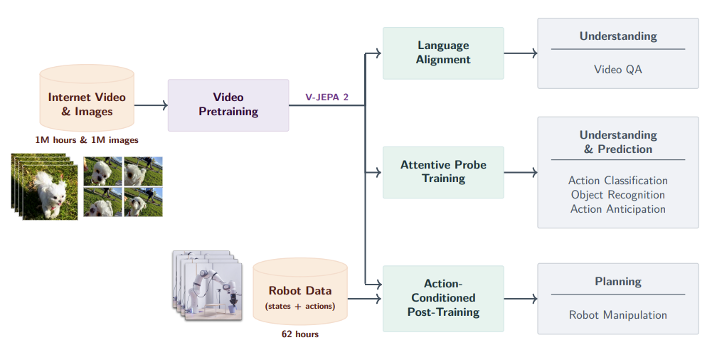
Remarkably, this action-conditioned model can be trained with a very small amount of robot data, on the order of tens of hours, because the bulk of the visual and dynamical understanding has already been acquired during large-scale video pretraining. The action-conditioning phase essentially grounds the abstract dynamics learned from internet video into a specific embodied agent
APPLICATION 2: Zero-Shot Planning with V-JEPA-2-AC Planning with V-JEPA-2-AC is performed entirely in embedding space. A current observation is encoded into a latent state, and a goal image is encoded into the same latent space. The planner searches for a sequence of actions such that the predicted future embedding, obtained by rolling the latent dynamics forward, matches the goal embedding.
Explicit World Models
An explicit world model is able to reconstruct or predict future observations in the same modality as perception (e.g., pixels, point clouds, images) during imagined rollouts. Unlike implicit models, the model does not only reason in latent space, but explicitly generates what the agent would see if a certain action sequence were executed.
The agent can “imagine” future frames of the world, not just abstract symbols. Thinking by actually rendering the future, not just reasoning abstractly about it
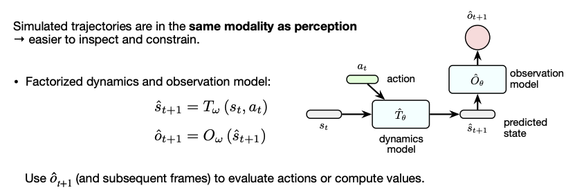
ARCHITECTURE Formally, the environment is modeled through two components. A dynamics model predicts how the internal state of the world evolves given the current state and an action, while an observation model maps that predicted state back to an observable quantity.
DINOV2 World Model
CORE IDEA In this paper by Zhou et al., 2024 illustrates how explicit world modeling can be combined with strong pretrained vision encoders.
- In this approach, observations are first encoded using DINOv2 representations, which provide rich and semantically meaningful visual features.
- A learned dynamics model (DINO-WM) then predicts how these representations evolve under actions
- a decoder reconstructs future observations from the predicted representations
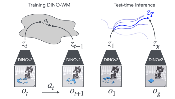
At test time, the model can roll forward from an initial observation under different action sequences and generate corresponding future visual trajectories. Because the predicted observations are explicit images, the agent can compare alternative futures visually or use them as input to downstream evaluation modules.
Diffusion World Models
CORE IDEA Diffusion world models extend explicit world modeling by using conditional diffusion processes to generate future observations. Rather than predicting a single deterministic outcome, these models learn a generative distribution over possible future trajectories conditioned on past observations and actions.
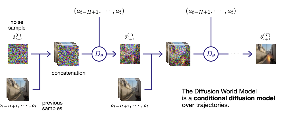
ARCHITECTURE In practice, a diffusion world model is trained to denoise future observations given a history of observations and a sequence of actions. Generation starts from noise and iteratively refines the sample until a plausible future observation, or even a full future trajectory, is produced.
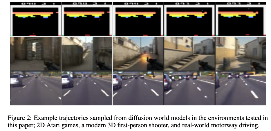
Because the model represents a distribution rather than a point estimate, multiple diverse futures can be sampled from the same initial state.
Instead of committing to a single imagined future, the agent reasons over a space of plausible futures.
Simulator Based World Models
CORE IDEA Instead of learning the environment dynamics and observation functions from data, they delegate the entire world modeling problem to an external simulator or to the real physical world itself. Instead of imagining future trajectories through a learned model, the agent evaluates actions by rolling them out inside the simulator.
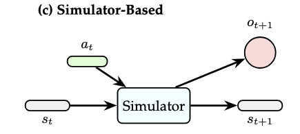
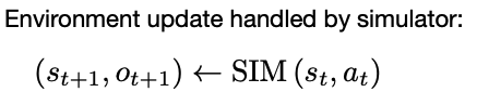
In this setting, the agent does not approximate the transition function \(T\) (to turn latent state into new latent state) or the observation function \(O\) (to turn latent state into pixel). Given a current state and an action, it simply queries the simulator, which returns the next state and the corresponding observation
The world model already exists; the agent only needs to query it.
SAPIEN
SAPien (Simulated Part-based Interactive Environment) is an open-source, physics-rich simulation platform designed specifically for robotics and embodied AI research
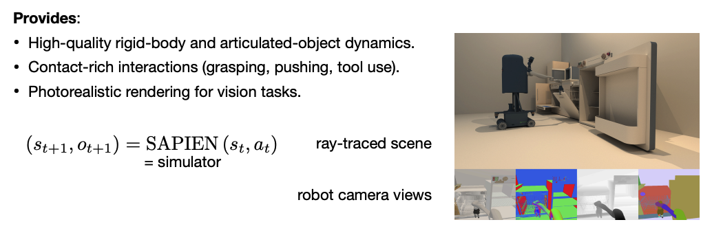
Learning happens on top of physics, not instead of it.
In practice, SAPien functions as a complete world model: given a state and an action, it deterministically (or stochastically, depending on configuration) produces the next state and observation. This makes it a natural backbone for research in robot learning, sim-to-real transfer, and vision-based control.
Instruction Driven
CORE IDEA Instruction-driven/hybrid world models are models that can be updated, constrained, or corrected via instructions, manuals, or on-the-fly rule discovery.
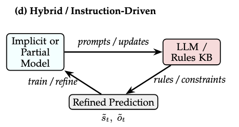
- A partial implicit or explicit model handles latent dynamics and perception, so state transition. But before completing the state transition it calls an external component
- an external reasoning component is typically an LLM or a structured rule base that is either updated and applied or prompted → it proposes constraints or checks consistency
- therefore, we improve via these suggestion the previously predicted state by latent dynamic
The world model is no longer only learned; it is instructed. Therefore is hybrid.
WHEN TO APPLY This hybrid setup is particularly powerful in environments where rules are known, partially known, or can be described linguistically, such as games, simulated worlds, or structured physical environments.
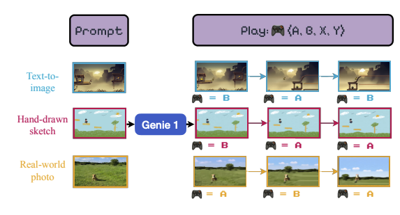
Genie: Instruction-Driven Generation of Playable Worlds
CORE IDEA Given a text prompt, Genie can generate dynamic, navigable worlds that respond in real time to user actions. The first prompt (sunny medieval village) generate the observed world via the world model, the other model the interactions that will happen.
ARCHITECTURE In Genie:
- the implicit or partial model corresponds to the autoregressive world model that predicts the next frame (or latent representation of the next frame) given the full prior trajectory and the current user action.
- External Reasoner During interaction, additional prompts or implicit instructions—such as player actions (move forward, turn, jump)—continuously update the conditioning context of the implicit model.
Genie Family
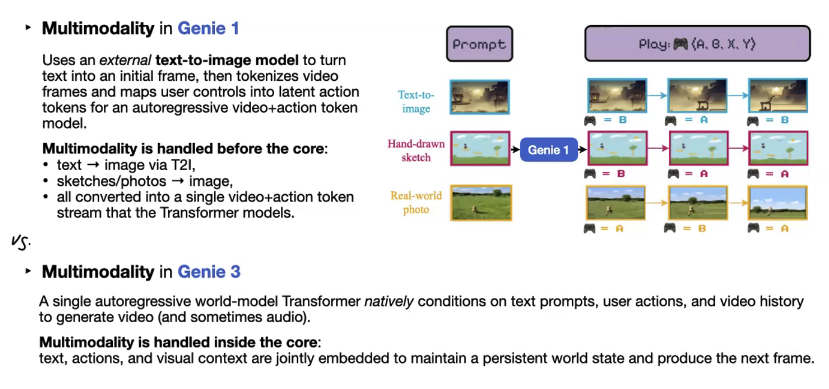
GENIE 1 introduces instruction-driven world modeling by combining a spatiotemporal video tokenizer with a latent action model. That is a Transformer-like dynamics model predicts the next frame (or latent tokens for the next frame), conditioned on: the past frames (or their tokens), the current user action, and often a text prompt.
Multimodality is handled outside the core model, with all inputs eventually mapped into a unified video–action token stream
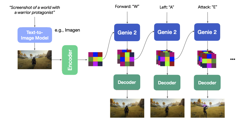
GENIE 2 Genie 2 advances this idea by using an autoregressive latent diffusion world model. Frames are encoded into a latent space and passed through a large Transformer dynamics model with causal masking. (classifier guidance allow to steer via text the generation of diffusion models)
same input(action) + state → GENIE → next state but now the state is latent, in GENIE 1 was pixel. Thereafter, a decoder maps it to observation in pixel space
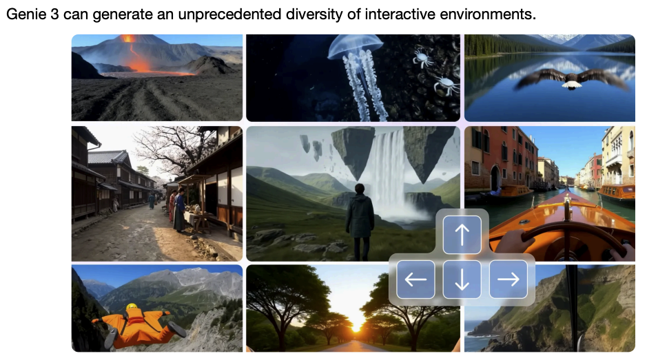
GENIE 3 Genie 3 further shifts toward real-time interaction. It is a frame-by-frame autoregressive world model that a_ttends to the full prior trajectory and maintains visual memory_. Genie 3 accepts direct text prompts and promptable world events, enabling richer instruction-driven control. While architectural details are not fully disclosed, it is explicitly optimized for interactive frame rates and persistent world state.
MULTIMODALITY COMPARISON In genie 1 everything is handled before the autoregressive world model. All text, image, and actions mapped to the same space on which world model is trained. In last one, Genie 3, instead everyhing is blended together natevily, there is not an embedder, which often times can be an information bottleneck
Cosmos Models for Physical AI
NVIDIA’s Cosmos World Foundation Model Platform provides an open-source, open-weight ecosystem for building high-fidelity digital twins of the physical world:
- very useful to address problem like data-scarcity in training robotics (physical AI) models
Within the Cosmos framework, different model families target different aspects of physical AI:
- Cosmos Predict focuses on
future state prediction, enabling forecasting and scenario planning by predicting how dynamic environments may evolve. - Cosmos Transfer provides multimodal simulation-to-simulation or simulation-to-real transfer, allowing policies and representations to generalize across environments.
- Cosmos Reason integrates vision-language reasoning to support higher-level understanding, commonsense reasoning, and decision-making in physical worlds.
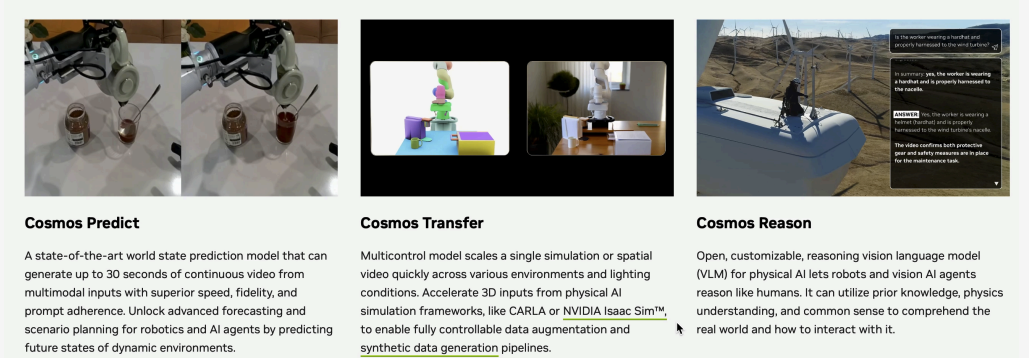
These models illustrate how instruction-driven world models can scale from research prototypes to production-grade systems, combining perception, dynamics, reasoning, and instruction-following into unified foundations for physical intelligence.